Twitter (X) Bot Detection: A Feature-Engineering Guide With Runnable Code

Twitter bot detection is the practice of scoring how likely an X account is automated by computing numeric features from its observable fields, its creation date, follow graph, posting cadence, engagement ratios, reply timing, and language, then combining those features into a probability you can act on. It is a classification problem, not a lookup. No single field decides the outcome, because every field produces false positives on its own. The method works when several independent features point the same way at once.

TL;DR: Do not ask "is this account a bot." Ask "how automated does this account look, which kind of bot is it, and how much does a mistake cost me here." Build five families of features (profile, temporal, engagement, network, language), fold them into a weighted score you can read line by line, then judge the score with base-rate math and a labeled evaluation set rather than raw accuracy. Everything below is runnable against a Twitter data API, with no model to train and no GPU.

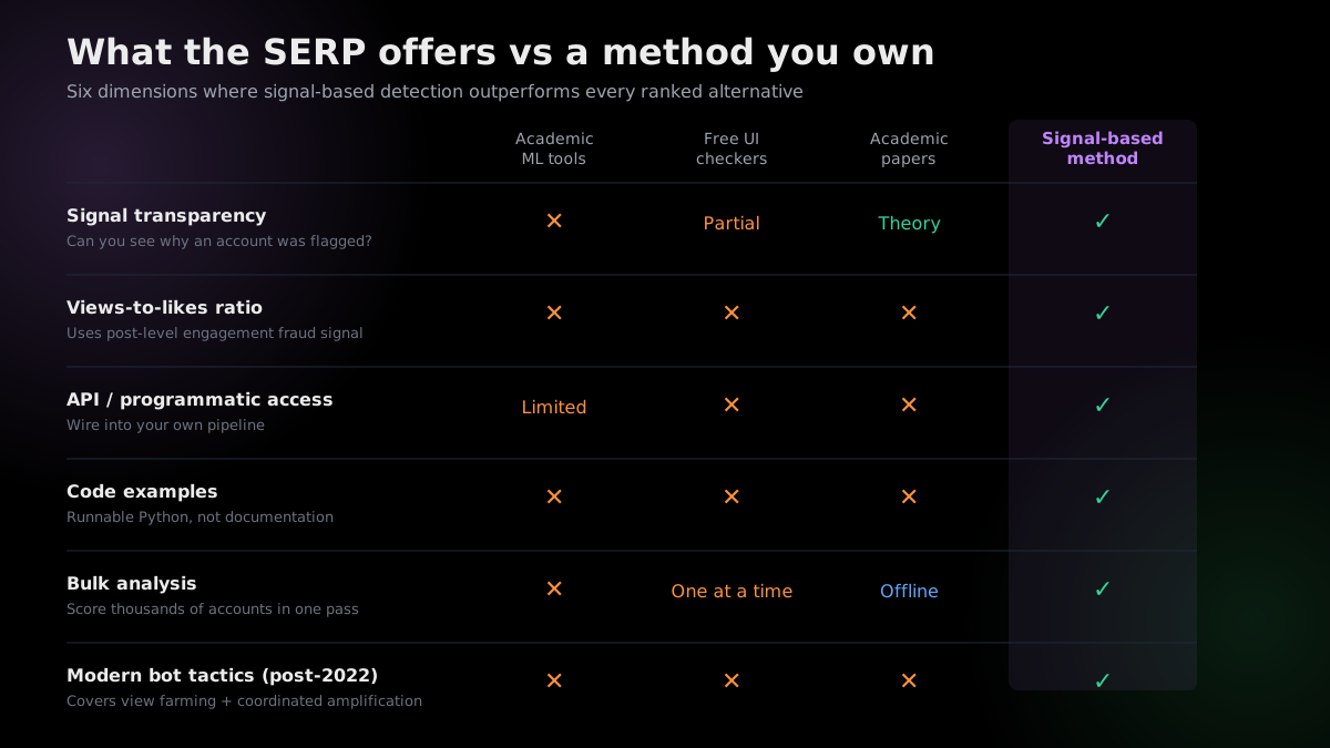
Most guides that rank for this query answer a single yes-or-no question about one account through a black box. That leaves the person actually building detection with nothing: no fields, no formulas, no way to run it across ten thousand followers, and no way to reason about how often the flag is wrong. This guide fills that gap. It treats detection the way a working data pipeline would, as feature extraction feeding a scoring model feeding an evaluation loop, and it hands you the code for each stage.

The instinct that brings most people here is usually correct. When a follower count balloons overnight or a mentions tab fills with near-identical replies, that is a real signal, not paranoia. The rest of this guide turns that instinct into something you can measure, reproduce, and defend.

A working definition, and why "is it a bot" is the wrong question

The word "bot" hides three separate questions that a good detector keeps apart.

The first is probability. Automation lives on a spectrum from a fully scripted account to a real person who schedules some posts through a tool. A detector should output a calibrated likelihood, not a binary label, because the accounts in the ambiguous middle are exactly where a binary forces you to guess.

The second is type. A follower-farm filler account that pads a count behaves nothing like a reply-spam bot, which behaves nothing like a coordinated astroturf network. Each type leaves a different fingerprint across the feature families, so a detector that only knows one type will miss the others entirely.

The third is cost. The threshold that is right for a brand-safety audit of a sponsorship deal, where a false accusation is expensive, is wrong for a spam filter, where letting one bot through is cheap and catching most of them matters more. The same feature set serves both, but the decision cutoff is a business choice, not a technical constant.

Hold those three apart and the design falls out naturally. You compute features once, produce a probability, read off which features fired to infer the type, and set the cutoff by what a mistake costs in your context. A model that collapses all three into one badge cannot do any of them well, which is precisely the failure mode of the one-click checkers.

Two structural facts make the field-based approach durable. The LOBO evaluation of Twitter bot classifiers trained a detector to over 97 percent accuracy on its own data and then showed it did not generalize to bot classes absent from that training set, which is the failure mode that matters in production, because the bots you have never seen are exactly the ones you are trying to catch. Work from the Stanford Internet Observatory on coordinated inauthentic behavior reaches a compatible conclusion: behavioral and network features age more slowly than trained classifiers because tactics move faster than any fixed training set. Observable fields do not rot the way model weights do, which is why a transparent feature pipeline is a better foundation than a frozen black box.

The six kinds of bots, and why one detector never catches them all

Before any code, get the taxonomy right, because the feature you weight heavily depends on which type you are hunting. Six classes cover almost everything you will meet on X.

Follower-farm filler. Cheap accounts whose only job is to pad a follower count. They barely post, follow far more than they are followed, and were often created in the same batch. They are the easiest class to catch from profile fields alone, and they are the class that produces the overnight follower floods real users keep reporting.

Why are hoards of bots suddenly following me? from r/Twitter

Reply-spam bots. Accounts that flood mentions with generic or scam replies, increasingly generated by a language model so the text reads plausibly. They give themselves away on timing and on the near-duplication of their output across many targets.

Engagement-farm amplifiers. Accounts bought to inflate a post through views, likes, or reposts. They deliver impressions by scrolling without engaging, which blows out the ratio between reach and reaction. This is the class the views-to-likes feature was built for.

Coordinated astroturf networks. Sets of accounts that individually pass a casual look but move as a group to push a narrative. They are invisible to per-account scoring and only surface at the network level, through creation-time cohorts and synchronized bursts.

AI-persona bots. Accounts that maintain a believable human persona with a stolen photo, an aged handle, and model-written posts. They defeat the naive visual checks entirely, and they are the reason language features have to be treated as weak tiebreakers rather than primaries.

Scam and phishing DM bots. Accounts that exist to slide into replies or messages with crypto, giveaway, or impersonation scams. They cluster on bio patterns, off-platform contact links, and coordinated timing.

The practical consequence is that a detector is really a small ensemble. A profile-only pass catches filler cheaply. Temporal and language features catch reply spam. Engagement ratios catch amplifiers. Network features catch astroturf. If you weight for one class and forget the others, your recall collapses on the classes you ignored, which is how a detector that looks accurate in a demo misses most of the real problem.

The feature space: five families of observable signals

Every feature you will compute belongs to one of five families. Naming the families matters, because it forces you to sample from all of them rather than piling five variants of the same idea into one score and calling it robust.

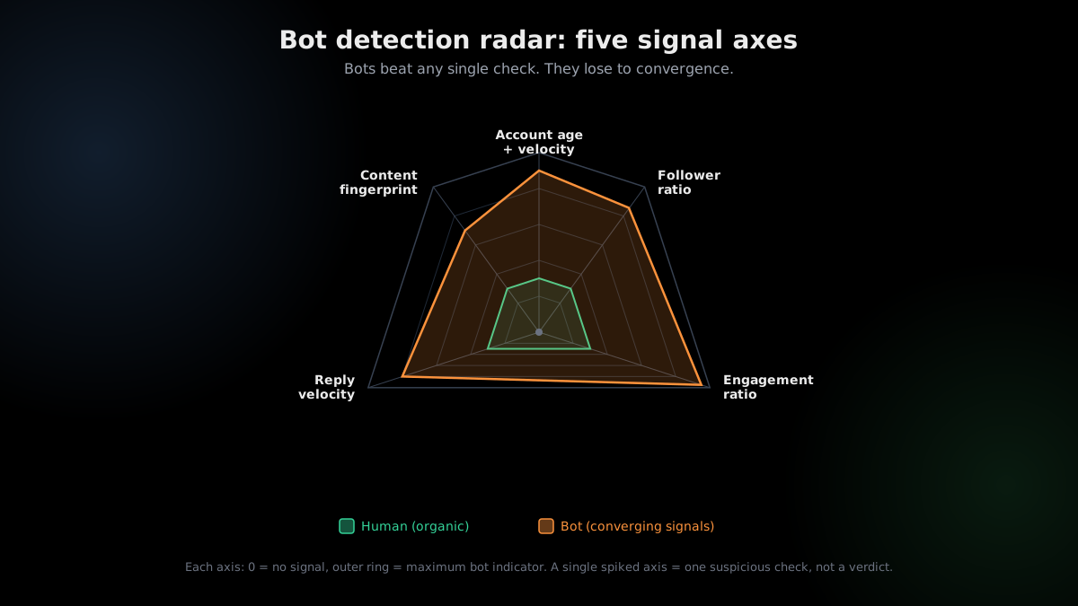
Profile and metadata features come straight off the account object with no extra request: account age in days, total post count, followers, following, whether the bio carries an off-platform contact link, whether the display name matches a template. These are the cheapest features, so they run first across a large list.

Temporal features describe when the account acts: the coefficient of variation of its inter-post intervals, the entropy of its posting hours, the median latency between a target post and its replies. Timing is expensive for an operator to fake convincingly, which makes this family disproportionately valuable.

Engagement-ratio features describe how reach relates to reaction: views to likes, likes to replies, reposts to likes, bookmarks to likes. Bought engagement distorts these ratios in characteristic ways that organic engagement does not.

Network and graph features describe the account's neighborhood: the creation-time cohort of its followers or of a post's engagers, the overlap between the follower sets of suspect accounts, the concentration of boosts from a small set of low-follower accounts. This family is the only one that catches coordination.

Content and language features describe what the account writes: exact-phrase repetition across its own posts, density of the stock vocabulary that language models overproduce, and structural tells like punctuation rate. This family is the noisiest, so it earns the lowest weight and serves as a tiebreaker.

The discipline is to draw at least one feature from each family before you weight anything. A score built from five profile features is fragile, because a single tactic, say aging the accounts, defeats all five at once. A score that spans families forces the operator to defeat several independent things simultaneously, which is far harder and far more expensive.

Feature engineering: turning raw fields into discriminative numbers

Raw fields are not features. followersCount on its own barely separates bots from people, because both new humans and filler bots can have few followers. The separation lives in derived quantities: ratios, rates, dispersions, and residuals against a baseline. Feature engineering is the step where you compute those, and it is where most of the discrimination actually comes from.

Start with a small extractor that pulls the account object and a window of recent posts, then derives the metadata and rate features. The code below uses a dataclass so every feature has a name you can inspect later, and it computes rates against active days rather than calendar age so a dormant-then-active account is not misread.

import os
import math
import statistics as st
from dataclasses import dataclass, asdict
from datetime import datetime, timezone

import requests

API_ROOT = "https://api.twitterapis.com"
AUTH = {"Authorization": f"Bearer {os.environ['TWITTERAPIS_KEY']}"}


def _iso(value: str) -> datetime:
    return datetime.fromisoformat(value.replace("Z", "+00:00"))


def account_object(handle: str) -> dict:
    resp = requests.get(
        f"{API_ROOT}/twitter/user/info",
        params={"userName": handle},
        headers=AUTH,
        timeout=20,
    )
    resp.raise_for_status()
    return resp.json()


def recent_window(handle: str, size: int = 40) -> list[dict]:
    resp = requests.get(
        f"{API_ROOT}/twitter/user/tweets",
        params={"userName": handle, "count": size},
        headers=AUTH,
        timeout=20,
    )
    resp.raise_for_status()
    return resp.json()["tweets"]


@dataclass
class MetaFeatures:
    age_days: int
    posts_total: int
    posts_per_day: float
    log_follow_ratio: float
    followers: int
    following: int
    has_offplatform_link: bool


def metadata_features(acct: dict) -> MetaFeatures:
    born = _iso(acct["createdAt"])
    age = max((datetime.now(timezone.utc) - born).days, 1)
    followers = acct.get("followersCount", 0)
    following = acct.get("followingCount", 0)
    # a symmetric, size-robust version of the follow-graph skew:
    # positive means following outweighs followers, zero means balanced
    ratio = math.log((following + 1) / (followers + 1))
    bio = (acct.get("description") or "").lower()
    off_link = any(tag in bio for tag in ("t.me/", "telegram", "whatsapp", "wa.me/"))
    return MetaFeatures(
        age_days=age,
        posts_total=acct.get("statusesCount", 0),
        posts_per_day=round(acct.get("statusesCount", 0) / age, 2),
        log_follow_ratio=round(ratio, 3),
        followers=followers,
        following=following,
        has_offplatform_link=off_link,
    )

Two engineering choices in that snippet do real work. Using a logarithm of the follow ratio turns an unbounded, skewed quantity into a symmetric one centered on zero, which behaves far better inside a linear score than a raw following / followers that explodes for zero-follower accounts. And flagging off-platform contact links in the bio is a cheap, high-precision feature for the scam-DM class specifically, since legitimate accounts rarely push Telegram or WhatsApp contact in their bio.

From here, every additional feature is another method on the same window of data. The point of engineering them as named, inspectable numbers is that when an account scores high later, you can read exactly which derived quantities drove the score, which is the property no black box gives you.

The engagement-ratio family in depth

Engagement ratios are the family that exposes bought reach, and they are worth a section on their own because they contain the single feature the older tools cannot compute. The public view count only became available on the X API in late 2022, after most academic detectors were built, so any model that predates it is structurally blind to view farming.

The mechanism is simple and mechanical. When someone buys reach, automated accounts deliver impressions by scrolling past a post, but they withhold the like, because liking at scale is what gets accounts caught in a sweep. Views climb while likes stay flat, and the ratio between them blows open. Organic posts behave the opposite way: a post that genuinely earns a hundred thousand views earned them through engagement, so likes scale roughly with reach.

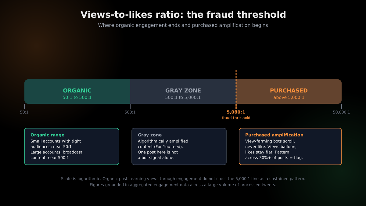
The reference band below is a working model, not a published constant. Treat it as a starting threshold you calibrate against your own labeled data, and never as a single-trigger verdict.

Methodology note: the roughly 50-to-500 organic views-to-likes band and the roughly 5,000-to-1 flag line are presented as an illustrative working model for how bought impressions distort the ratio. They are order-of-magnitude guidance for setting an initial threshold, they vary with account size and content type, and they require convergence with other features before they mean anything. Calibrate them against a hand-labeled sample for your own use case rather than treating them as fixed.

The extractor below computes several engagement ratios per post, not just views to likes, because the secondary ratios catch amplifiers that buy a mix of interactions rather than raw views alone.

@dataclass
class EngagementFeatures:
    posts_scored: int
    farm_share: float
    median_view_like: float
    median_reply_like: float


def engagement_features(posts: list[dict], min_views: int = 1000,
                        flag_line: int = 5000) -> EngagementFeatures:
    view_like, reply_like, farmed = [], [], 0
    scored = [p for p in posts if (p.get("viewCount") or 0) >= min_views]
    for p in scored:
        views = p.get("viewCount") or 0
        likes = (p.get("likeCount") or 0) + 1   # smooth zero-like posts
        replies = (p.get("replyCount") or 0) + 1
        vl = views / likes
        view_like.append(vl)
        reply_like.append(replies / likes)
        if vl > flag_line:
            farmed += 1
    denom = max(len(scored), 1)
    return EngagementFeatures(
        posts_scored=len(scored),
        farm_share=round(farmed / denom, 2),
        median_view_like=round(st.median(view_like), 1) if view_like else 0.0,
        median_reply_like=round(st.median(reply_like), 2) if reply_like else 0.0,
    )

Two guards keep this honest. Posts under a thousand views are dropped, because thin posts throw wild ratios from rounding and carry no information. And the account-level feature is the share of its posts that cross the flag line, never a single post, because any real account can catch one viral-but-unliked tweet. A pattern of high-ratio posts is the tell; one outlier is noise.

The reply-spam class shows up here too, from the other side. When an account's own posts draw almost no replies relative to likes across a whole window, or when a target's mentions fill with generic automated replies, the engagement shape is off in a way a human eye registers as "this feels fake" and these ratios make measurable. The frustration is common enough that large accounts have started closing their replies entirely rather than fight it, because AI reply bots have made an open mentions tab untenable.

https://x.com/signulll/status/2073154745578008867

Temporal features: the clock is the hardest thing to fake

If engagement ratios are the family that catches bought reach, temporal features are the family that catches automation itself, because timing is the attribute an operator finds hardest to fake convincingly at scale. A person posts in bursts separated by long silences, sleeps on a rough schedule, and replies with human latency. Naive automation posts at near-constant intervals, around the clock, and answers within seconds.

Three temporal features do most of the work. The first is burstiness, the coefficient of variation of the gaps between consecutive posts. Human activity is bursty, with a high spread of intervals; metronomic automation has a low spread. The second is posting-hour entropy, how evenly an account's activity is spread across the twenty-four hours of the day. A human clusters into waking hours; an always-on bot spreads flat, which reads as high entropy, while a scripted-schedule bot collapses into a few exact slots, which reads as suspiciously low entropy. The third is reply latency, the median gap between a target post and the replies to it, which flags amplification bots that fire the moment a post lands.

def _intervals(times: list[datetime]) -> list[float]:
    ordered = sorted(times)
    return [(ordered[i] - ordered[i - 1]).total_seconds()
            for i in range(1, len(ordered))]


@dataclass
class TemporalFeatures:
    burstiness: float
    hour_entropy: float
    posts_in_window: int


def temporal_features(posts: list[dict]) -> TemporalFeatures:
    times = [_iso(p["createdAt"]) for p in posts if p.get("createdAt")]
    gaps = _intervals(times)
    if len(gaps) >= 2 and st.mean(gaps) > 0:
        cv = st.pstdev(gaps) / st.mean(gaps)     # coefficient of variation
    else:
        cv = 0.0

    # Shannon entropy of the posting-hour distribution, normalized to 0..1
    hours = [t.hour for t in times]
    entropy = 0.0
    if hours:
        for h in set(hours):
            share = hours.count(h) / len(hours)
            entropy -= share * math.log(share, 2)
        entropy /= math.log(24, 2)

    return TemporalFeatures(
        burstiness=round(cv, 2),
        hour_entropy=round(entropy, 2),
        posts_in_window=len(times),
    )


def reply_latency(parent_iso: str, replies: list[dict]) -> dict:
    parent = _iso(parent_iso)
    gaps = [(_iso(r["createdAt"]) - parent).total_seconds()
            for r in replies if r.get("createdAt")]
    fast = [g for g in gaps if 0 <= g < 30]
    return {
        "replies_seen": len(gaps),
        "median_latency_s": round(st.median(gaps), 1) if gaps else None,
        "fast_reply_share": round(len(fast) / max(len(gaps), 1), 2),
    }


def pull_replies(post_id: str, size: int = 100) -> list[dict]:
    resp = requests.get(
        f"{API_ROOT}/twitter/tweet/replies",
        params={"tweetId": post_id, "count": size},
        headers=AUTH,
        timeout=20,
    )
    resp.raise_for_status()
    return resp.json()["replies"]

The interpretation takes a little care, because both very low and very high posting-hour entropy can be suspicious for different bot types, so this feature is best read alongside burstiness rather than alone. A scripted account posting at exact clock intervals shows low burstiness and low entropy together, a combination that is almost impossible for a human to produce. An always-on amplification account shows flat, high entropy with fast reply latency. Reading the two together separates the scheduler bot from the swarm bot, which is a distinction a single flat "posts fast" signal cannot make.

Temporal features cost more than metadata, since reply latency needs a replies call per post, so they run after the cheap profile pass has narrowed the field. The Twitter API rate limit guide covers backoff for sustained reply-fetch jobs, and the python twitter API tutorial covers the timestamp-parsing patterns these features depend on.

Content and language features: the noisy but useful family

The last per-account family reads what the account writes, and it is worth building even though it is the weakest, because it is the family that catches the AI-persona and reply-spam classes when the metadata looks clean. The rule to internalize first is that these features carry the lowest weight in the score, because human writing varies enormously and plenty of real people write in ways that trip a naive content check. Language features are tiebreakers that push a borderline account over the line, never a primary you convict on.

Three content features hold up reasonably well. The first is exact-phrase repetition, the share of an account's posts that duplicate each other verbatim or near-verbatim. Template-driven bots repeat sentences more often than a human ever would, and reply-spam bots reuse the same lines across many different targets. The second is stock-vocabulary density, the rate at which the account uses the words that language models overproduce relative to normal speech. The third is a structural one, punctuation and formatting regularity, since some automated text is unnaturally uniform in how it opens and closes.

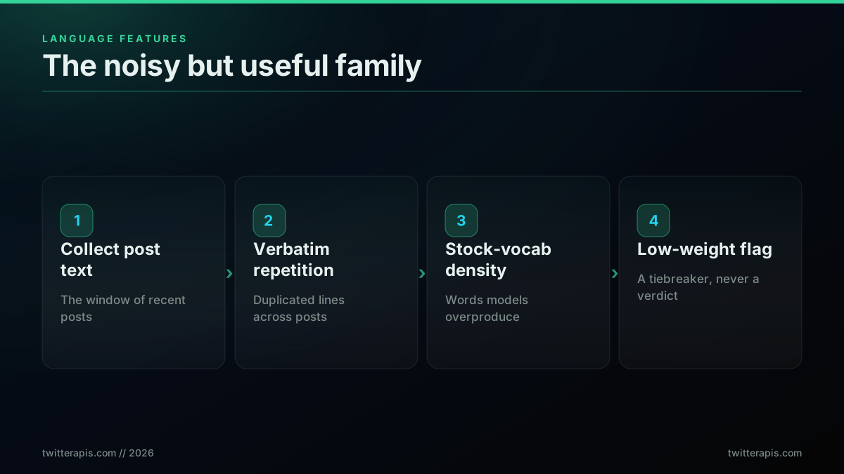
The extractor below closes the loop on the language_flags call the scorecard uses. It stays deliberately conservative, firing only when repetition or vocabulary density is well above a normal baseline, so it rarely fires on a real account.

import re

STOCK_VOCAB = {
    "delve", "tapestry", "multifaceted", "holistic", "seamless",
    "robust", "leverage", "elevate", "unlock", "utilize", "furthermore",
}


def language_flags(posts: list[dict]) -> dict:
    texts = [p.get("text", "") for p in posts if p.get("text")]
    if not texts:
        return {"repeat_rate": 0.0, "stock_rate": 0.0, "language_flag": False}

    normalized = [re.sub(r"\s+", " ", t.strip().lower()) for t in texts]
    duplicates = sum(count - 1 for count in Counter(normalized).values() if count > 1)
    repeat_rate = duplicates / len(normalized)

    words = re.findall(r"[a-z']+", " ".join(normalized))
    stock_hits = sum(1 for w in words if w in STOCK_VOCAB)
    stock_rate = stock_hits / max(len(words), 1)

    return {
        "repeat_rate": round(repeat_rate, 2),
        "stock_rate": round(stock_rate, 3),
        "language_flag": repeat_rate > 0.15 or stock_rate > 0.01,
    }

The reason to keep this family in the score at all, despite its noise, is that it is the only family that looks at content rather than structure, and content is where an AI-persona bot that has aged its account and warmed its follow graph still has to say something. The catch, covered in the failure-modes section, is that a capable language model defeats these features outright, which is why they never carry more than a single point. For deeper content analysis than a repetition check, the Twitter sentiment analysis in Python walkthrough and the complete Twitter API tutorial cover the text-processing patterns, and X frames the whole distinction between declared automation and deceptive behavior in its platform manipulation policy, which is the behavior the content family targets.

Network features: detecting the farm, not the sheep

Per-account scoring, no matter how many features it stacks, misses the most damaging pattern on the platform: coordination. A network of accounts that each pass a casual look can together push a narrative or inflate a post, and the only way to see it is to stop scoring accounts one at a time and start scoring the set.

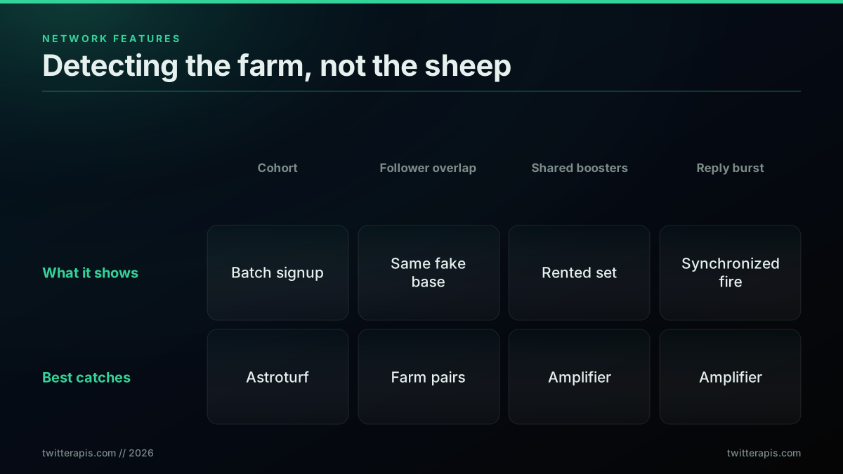
The question shifts from "is this account automated" to "do these accounts move as a group." Four network features carry most of the signal. Account-creation cohort concentration measures how many of a set's accounts were registered in the same narrow window; a real audience is created across years, a farm across weeks. Follower-set overlap measures how similar two suspect accounts' follower lists are, since farmed accounts often share large chunks of the same fake followers. Shared-booster concentration measures how much of a set of posts is boosted by the same small group of low-follower accounts. Synchronized reply bursts measure how tightly the set's replies cluster in time.

Cohort concentration is the strongest of the four and the cheapest to compute, since it needs only the creation date off each engager's profile. The function below buckets engagers by the month they were created and returns the share sitting in the single busiest bucket.

from collections import Counter


def cohort_concentration(engagers: list[dict]) -> dict:
    buckets = Counter()
    for e in engagers:
        born = _iso(e["createdAt"])
        buckets[(born.year, born.month)] += 1
    total = sum(buckets.values())
    peak = max(buckets.values()) / total if total else 0.0
    return {
        "engagers": total,
        "peak_cohort_share": round(peak, 2),
        "cohort_flag": peak > 0.4,
    }


def follower_set_overlap(followers_a: set[str], followers_b: set[str]) -> float:
    if not followers_a or not followers_b:
        return 0.0
    inter = len(followers_a & followers_b)
    union = len(followers_a | followers_b)
    return round(inter / union, 3)   # Jaccard similarity

When more than roughly forty percent of a post's engagers were created in a single month, that is not how organic audiences form; it is how a batch of accounts gets registered. Pair cohort concentration with synchronized reply bursts across the same set and you have a coordinated-amplification detector, the network-level complement to the per-account score. The follower-set overlap function extends this to pairs of suspect accounts: two accounts sharing most of their followers are almost certainly from the same farm, since real accounts built independent audiences.

The third network feature, shared-booster concentration, is worth its own function because it catches the amplification farm that cohort concentration misses when the accounts are aged rather than freshly minted. The idea is bipartite: build the mapping from each booster account to the set of posts it engaged, then find the boosters that show up across an implausible number of the target posts. A handful of accounts that reliably like or repost everything a target puts out, especially low-follower accounts, is a rented amplification set, not an organic audience.

def shared_booster_concentration(post_to_engagers: dict[str, list[str]]) -> dict:
    # post_to_engagers maps a post id to the list of account ids that boosted it
    booster_hits = Counter()
    for engagers in post_to_engagers.values():
        for account_id in set(engagers):
            booster_hits[account_id] += 1
    n_posts = max(len(post_to_engagers), 1)
    # boosters that engaged more than 60% of the target's posts
    persistent = [acct for acct, hits in booster_hits.items()
                  if hits / n_posts > 0.6]
    return {
        "unique_boosters": len(booster_hits),
        "persistent_boosters": len(persistent),
        "persistent_share": round(len(persistent) / max(len(booster_hits), 1), 3),
    }

Run this over a target's recent posts and a high persistent share is a strong coordination signal, because a real audience engages selectively while a rented one engages everything. Combined with cohort concentration and reply-burst timing, the three network features triangulate a farm from three independent angles, which is the same convergence discipline the per-account score uses, applied to a set.

The follower floods that individual users report are usually the visible edge of exactly this kind of batch registration. A synchronized wave of new followers is a cohort, and the same math that unmasks a coordinated amplification set unmasks a follower farm.

Inundated by bot followers too? from r/Twitter

For a longer look at how these networks are built and run, this long-form investigation into how bot and troll farms actually operate is a useful primer on the coordination patterns the network features are designed to quantify. These are the features that unmask a coordinated set rather than a single account:

https://www.youtube.com/watch?v=GZ5XN_mJE8Y

Pulling the engager set and the follower lists this section needs means reading many accounts at once, which the tweet history scraping guide and the export Twitter followers guide cover in depth.

From features to a score: three scoring models

You have five families of features. Now they have to become one number, and there are three levels of sophistication for doing that, each right for a different stage.

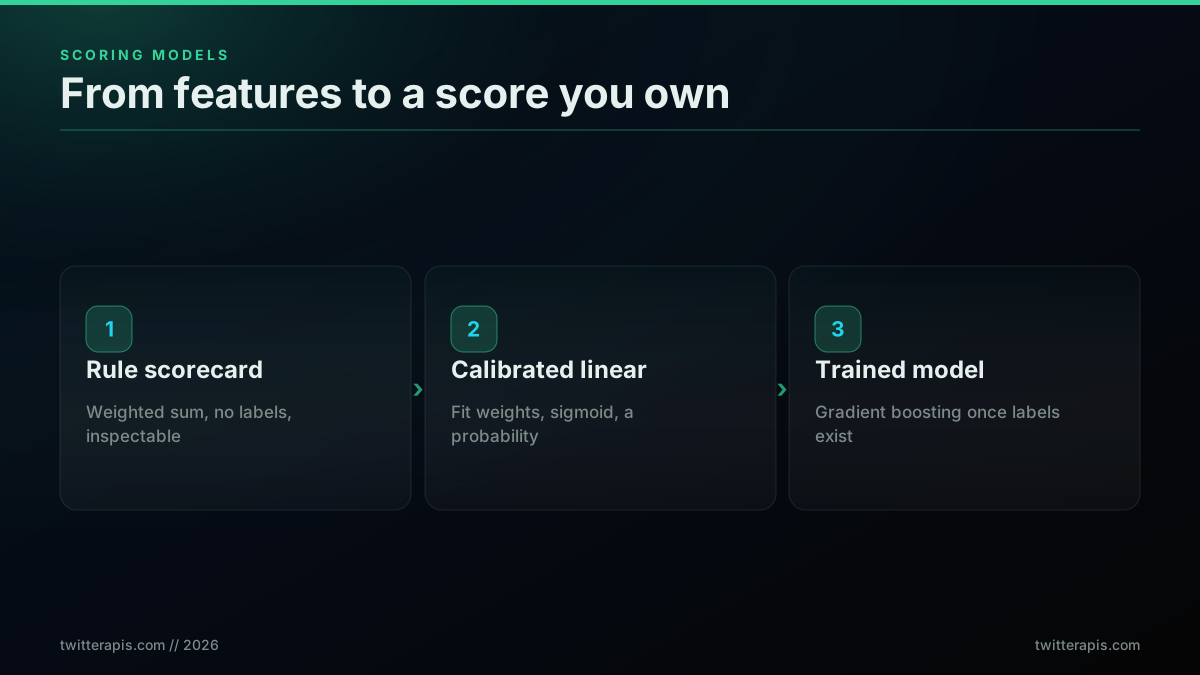
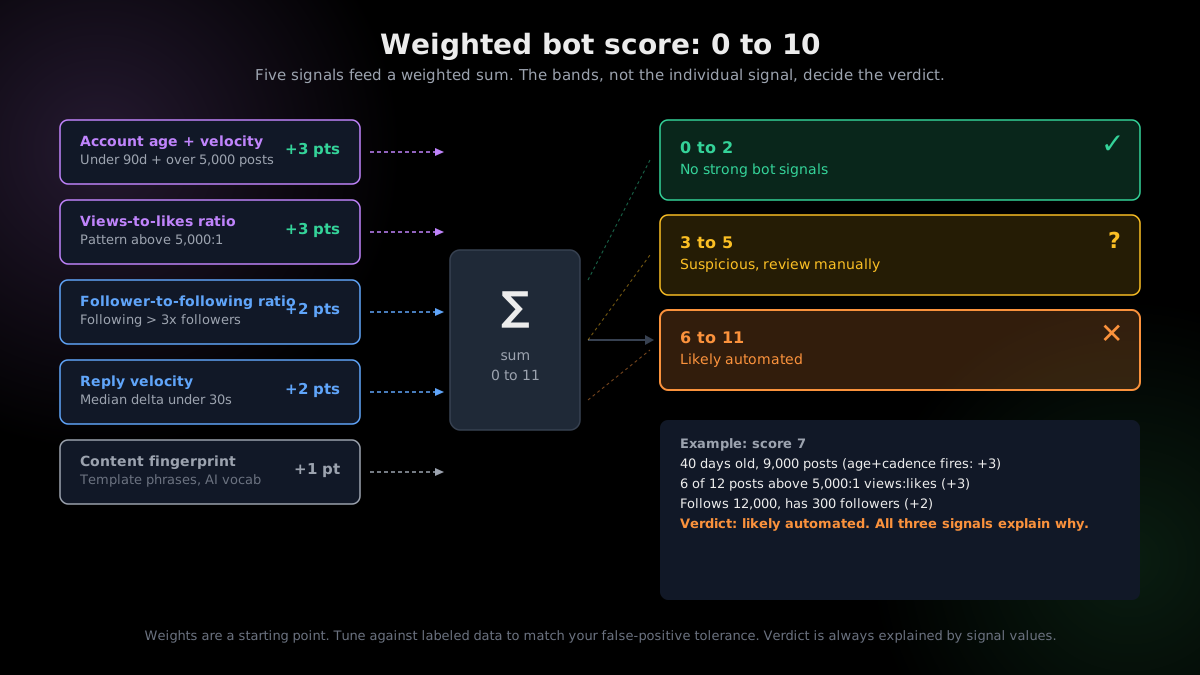
Model one: the rule scorecard. Assign each feature a weight by how much it discriminates, sum the weights of the features that cross their threshold, and read the total against bands. This is the right first build because every decision is inspectable and it needs no labeled data to stand up. The class below composes the extractors from the earlier sections.

class BotScorecard:
    WEIGHTS = {
        "farm_share": 3,        # engagement family, high confidence
        "young_and_loud": 3,    # profile family, high confidence
        "skew": 2,              # profile family, medium
        "metronomic": 2,        # temporal family, medium
        "language": 1,          # content family, low, tiebreaker only
    }

    def __init__(self, acct: dict, posts: list[dict]):
        self.meta = metadata_features(acct)
        self.eng = engagement_features(posts)
        self.temp = temporal_features(posts)
        self.lang = language_flags(posts)

    def _fired(self) -> dict:
        return {
            "farm_share": self.eng.farm_share > 0.3,
            "young_and_loud": self.meta.age_days < 90 and self.meta.posts_total > 5000,
            "skew": self.meta.log_follow_ratio > 1.1 and self.meta.following > 200,
            "metronomic": self.temp.burstiness < 0.4 and self.temp.posts_in_window >= 8,
            "language": self.lang["language_flag"],
        }

    def score(self) -> dict:
        fired = self._fired()
        total = sum(w for k, w in self.WEIGHTS.items() if fired[k])
        if total >= 6:
            band = "likely automated"
        elif total >= 3:
            band = "suspicious, review by hand"
        else:
            band = "no strong automation signal"
        return {"score": total, "band": band, "fired": fired,
                "features": {"meta": asdict(self.meta), "eng": asdict(self.eng),
                             "temporal": asdict(self.temp)}}

Notice that the scorecard returns the fired flags and the raw feature values alongside the score. When an account scores seven, you can read that it is forty days old with nine thousand posts, its log follow ratio is high at volume, and a third of its posts cross the farm line. That is an explanation a person can check, not a verdict handed down from a model, and the explanation is the feature that keeps the whole method trustworthy.

Model two: the calibrated linear score. The scorecard's weights are integers you guessed. The next step is to fit them against a small hand-labeled set and pass the result through a sigmoid so the output is a probability between zero and one rather than a raw count. You do not need a machine-learning library for this; a few dozen labeled accounts and least-squares on the feature matrix, or even manual weight tuning against a confusion matrix, is enough to move from a guess to a calibration.

def logistic(x: float) -> float:
    return 1.0 / (1.0 + math.exp(-x))


def calibrated_probability(features: dict, weights: dict, bias: float) -> float:
    # features and weights are aligned dicts of numeric feature -> coefficient
    z = bias + sum(weights.get(k, 0.0) * v for k, v in features.items())
    return round(logistic(z), 3)

The value of the calibrated version is that a probability composes. You can set different cutoffs for different jobs against the same score, feed the probability into a downstream ranking, and report a number that means something rather than a raw tally whose scale you invented.

Model three: the trained classifier. Once you have a few hundred labels, a gradient-boosted tree over the same feature vector will usually beat a hand-tuned linear score, because it captures interactions between features that a linear model cannot. This is where machine learning earns its place, and only here. The operational cost is real: you now own a training set that has to be refreshed as tactics drift, and the model becomes a black box unless you keep the feature attributions. The honest guidance is to graduate to a trained model when precision on the linear score plateaus and you have the labels to support it, not before.

Whichever model you run, the point holds, and a founder who has watched it from the product side makes the same case: automation reveals itself across a whole pattern of behavior over time, not in any one post, which is exactly why the score sums many features rather than trusting a single field.

https://x.com/Shpigford/status/2030356651027419572

A worked example: scoring one account end to end

Theory is easier to trust once you watch it run, so walk a single account through the whole pipeline. The driver below reads the profile and a window of posts, runs the scorecard, and prints the fired features alongside the band, which is the output shape you want in production because it is auditable.

def run(handle: str) -> dict:
    acct = account_object(handle)
    posts = recent_window(handle, size=40)
    result = BotScorecard(acct, posts).score()
    print(f"@{handle}: {result['band']} (score {result['score']}/11)")
    for name, fired in result["fired"].items():
        if fired:
            print(f"  fired: {name}")
    return result


run("someaccount")

Now read a concrete, hypothetical result to see how the bands behave. Imagine the scorecard returns a score of eight for an account. Reading the feature dump, you find it is fifty-one days old with eleven thousand posts, which fires young_and_loud for three points. Its log follow ratio is well above one at a following count in the thousands, which fires skew for two points. Its burstiness is 0.31 across a full window of forty posts, which fires metronomic for two points. And a small language flag adds one. Engagement is clean, so farm_share does not fire. The account lands in the likely-automated band, and crucially you can see that the verdict rests on the profile and temporal families converging, not on any single field. That is a filler or scheduler bot, not an amplifier, and the fired flags told you which type without you asking a separate question.

Contrast that with an account that scores three. It fires only farm_share, because a third of its posts cross the view-farm line, but its age, follow graph, and cadence are all normal. That single high-confidence flag lands it in the suspicious band, which is exactly right: something is off with its reach, but the account itself may be a real person whose posts were amplified by a bought network rather than a bot itself. The score refuses to convict, and it points you at the engagement family to investigate. This is the payoff of a transparent, family-spanning score. It does not just output a number; it tells you where to look next.

An account that scores zero or one, with no families converging, is cleared, and you move on without spending a per-post deep check on it. That triage, running the cheap families first and only deep-checking the accounts that already look off, is what makes the whole thing affordable at scale, which the production section formalizes. Caching profile responses across the run keeps the cost down further, a pattern the TwitterAPIs best practices guide covers, and if you are scoring accounts around a live event or trending topic, the Twitter trends API guide covers narrowing the set to the accounts actually engaging the moment.

One implementation note worth stating plainly: the view count that powers the engagement family is a relatively recent field, and X documents how view counts are surfaced, so if you are reading from a source that does not expose it, the whole engagement family goes dark and you lean harder on the profile, temporal, and network families instead. The method degrades gracefully; it does not break.

Base rates, precision, and the false-positive trap

Here is the math almost no bot-detection guide shows, and it is the math that separates a detector you can trust from one that quietly floods you with false accusations. The problem is base rates.

Suppose you scan a follower list where five percent of the accounts are genuinely bots. You build a detector with ninety percent recall, meaning it catches ninety percent of the real bots, and ninety-five percent specificity, meaning it correctly clears ninety-five percent of the real people. Those sound like strong numbers. Now run the confusion matrix on ten thousand accounts.

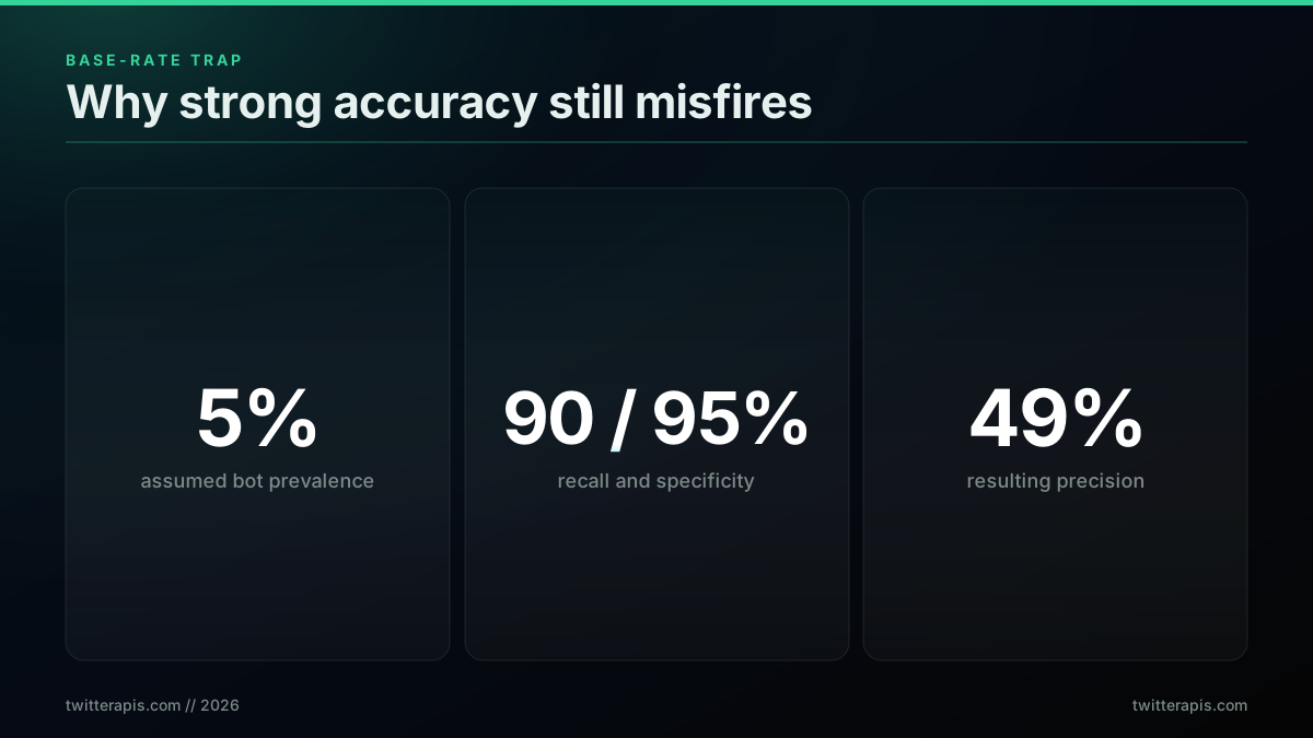
Of the ten thousand accounts, five hundred are bots and nine thousand five hundred are people. Ninety percent recall catches four hundred fifty of the bots. Five percent of the nine thousand five hundred people, which is four hundred seventy-five accounts, get flagged wrongly. So your flags total nine hundred twenty-five accounts, of which only four hundred fifty are real bots. Precision is four hundred fifty over nine hundred twenty-five, which is about forty-nine percent. Half of everything the detector flags is a real person, despite recall and specificity that both looked excellent.

Metric	Value	What it means
Bot prevalence	5%	Bots are rare relative to real accounts
Recall	90%	Share of real bots the detector catches
Specificity	95%	Share of real people the detector clears
Flags on 10,000 accounts	925	450 true bots plus 475 false alarms
Precision	~49%	Share of flags that are actually bots

The lesson is that at low prevalence, specificity dominates precision, and recall is almost a distraction. Pushing specificity from ninety-five to ninety-nine percent, by demanding more converging features before you flag, cuts the false alarms from four hundred seventy-five to ninety-five and lifts precision from forty-nine to about eighty-three percent, a far bigger win than any improvement in recall could deliver. This is the quantitative reason the whole method insists on convergence: every additional independent feature you require raises specificity, and specificity is what buys you precision when the thing you are hunting is rare. The Pew Research analysis of automated accounts sharing links on Twitter is a useful reference point for how prevalence varies by context, and Emilio Ferrara and colleagues' survey of social bots documents why single-feature detectors were always destined to generalize poorly.

Evaluation: building a labeled set and reading the numbers

A detector you have not evaluated is a detector you should not trust. Evaluation is not optional polish; it is the step that tells you where to set the cutoff and how often the flag is wrong. It has three parts.

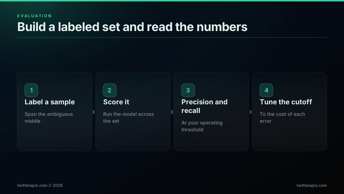
Build a labeled set. Sample accounts in a way that reflects the population you will run against, not a convenient batch of obvious bots. Hand-label each as bot or human using every signal available, including a manual review of the profile and recent posts. A few hundred labels is enough to start; the goal is a set that spans the ambiguous middle, not just the easy cases, because the easy cases tell you nothing about where your threshold should sit.

Compute the metrics that matter. Run your score across the labeled set and build the confusion matrix. Precision and recall at your chosen threshold matter far more than accuracy, for the base-rate reason from the previous section. Precision at the top of the ranked list, precision at k, is often the most operationally useful number, because in practice you review the highest-scoring accounts first.

def evaluate(scored: list[tuple[float, bool]], threshold: float) -> dict:
    # scored = list of (predicted_probability, is_bot_label)
    tp = sum(1 for p, y in scored if p >= threshold and y)
    fp = sum(1 for p, y in scored if p >= threshold and not y)
    fn = sum(1 for p, y in scored if p < threshold and y)
    precision = tp / (tp + fp) if (tp + fp) else 0.0
    recall = tp / (tp + fn) if (tp + fn) else 0.0
    f1 = (2 * precision * recall / (precision + recall)
          if (precision + recall) else 0.0)
    return {"threshold": threshold, "precision": round(precision, 3),
            "recall": round(recall, 3), "f1": round(f1, 3),
            "flags": tp + fp, "true_bots_caught": tp}


def sweep_thresholds(scored: list[tuple[float, bool]]) -> list[dict]:
    return [evaluate(scored, t / 10) for t in range(1, 10)]

Tune the threshold to the cost. Sweep the cutoff across its range and read the precision-recall tradeoff. A brand-safety audit picks a high threshold that keeps precision near the top, accepting that it misses some bots, because a false accusation is expensive. A spam filter picks a lower threshold that keeps recall high, accepting more false alarms, because letting bots through is the costlier error. The right cutoff is wherever the ratio of the two error costs balances for your job, and the sweep is what lets you find it deliberately rather than by feel.

The last piece is drift. Bot tactics change, so a threshold tuned in one quarter degrades in the next. Re-label a fresh sample on a regular cadence, re-run the sweep, and watch precision at your operating threshold over time. When it slips, your features or your cutoff need attention. Skipping this step is how a detector that was accurate at launch silently rots into a nuisance.

Failure modes and the adversary

Every feature in this guide can be defeated, and a serious operator will try. Knowing how each one breaks is what keeps you from over-trusting a score, and it is the difference between a detector that degrades gracefully and one that fails silently.

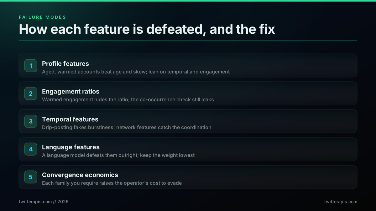
Take the families in turn. Profile features fall to aged and warmed accounts: an operator who buys handles that are years old with organic-looking follow graphs defeats age and skew entirely. The mitigation is to lean harder on temporal and engagement features, which aging does not fix. Engagement ratios fall to warmed engagement, where the operator buys a realistic mix of likes and replies alongside views so the ratios stay in the organic band. The mitigation is the co-occurrence check: warmed engagement is expensive, so it rarely covers a whole posting history, and the residual posts still leak. Temporal features fall to drip-posting, where a bot spaces its output with randomized delays to fake burstiness and confines itself to waking hours to fake a circadian rhythm. The mitigation is network features, because coordinating drip-posting across a farm reintroduces the synchronization the network family catches. Language features fall hardest and fastest, because a language model produces varied, human-sounding text that defeats phrase-repetition and stock-vocabulary checks outright, which is exactly why this family carries the lowest weight and never convicts alone.

There is a deeper adversarial point about cost asymmetry. The reason to require convergence is not only statistical precision; it is economics. Each independent feature you demand raises the operator's cost to evade, because they now have to fake several unrelated things at once. Aging accounts, warming engagement, drip-posting on a human schedule, and coordinating it all across a network without leaving a cohort signature is expensive, and expense is the real constraint on bot operations. A detector that forces the adversary to spend more than the amplification is worth has done its job, even if a determined, well-funded operator can still beat any single feature.

Concept drift ties it together. The tactics that defeat your features this quarter are the tactics your labeled set has to include next quarter. A detector is not a thing you build once; it is a loop you maintain, and the failure modes are the map of where the loop needs the most attention.

Edge cases: the legitimate accounts these features flag

A detector is only as trustworthy as its handling of the real accounts that happen to look automated, and there are several well-known classes of person who trip individual features while being entirely human. Knowing them is what stops you from acting on a single flag, and it is the practical face of the convergence rule.

A journalist or analyst live-tweeting an event posts dozens of times in an hour with low burstiness and fast reply latency, which fires the temporal features. What clears them is that their follow graph, engagement ratios, and account age are all normal, so the score never reaches the automated band. A brand or media account run by a social team posts on a schedule through a tool, which can fire the metronomic feature, but again the other families clear it. A genuinely new power-user builds a high post count fast while young, which fires young_and_loud, yet has organic engagement and a normal follow graph. An account recovering from a spam purge shows a temporarily skewed follow ratio for weeks after the platform removed its fake followers, which is the cruel irony that the victim of a bot problem can briefly look like a bot. And a creator who ran a giveaway attracts a burst of low-quality followers created in a narrow window, which can fire cohort concentration even though the creator did nothing wrong.

The pattern across all of these is identical: one feature fires, the rest do not, and the score stays low because no families converge. This is not an accident of the thresholds; it is the entire design goal. Every one of these accounts would be a false positive under a single-signal detector, and every one of them is correctly cleared by a score that requires several independent families to agree. When you present a flag to a human reviewer, presenting it as "fired on temporal only, cleared on profile, engagement, and network" is what lets them dismiss it in seconds. The interpretability is not a nicety; it is what makes the false-positive rate survivable in practice.

The operational rule that falls out of this is simple. A flag is the start of a review, never the end of one. A score of eight with four families converging is close to actionable on its own; a score of three on a single family is a prompt to look, not a verdict. Encoding that distinction into how you route flags, auto-actioning only the high-convergence cases and queuing the rest for a human, is what keeps the whole system from eroding trust the first time it wrongly accuses a real person.

Putting it in production: ordering, caching, and idempotency

Scoring one account is a demo. Auditing a whole follower list, yours or a prospect's, is the real job, and doing it at scale is an engineering problem as much as a detection problem. Three practices make it affordable and repeatable.

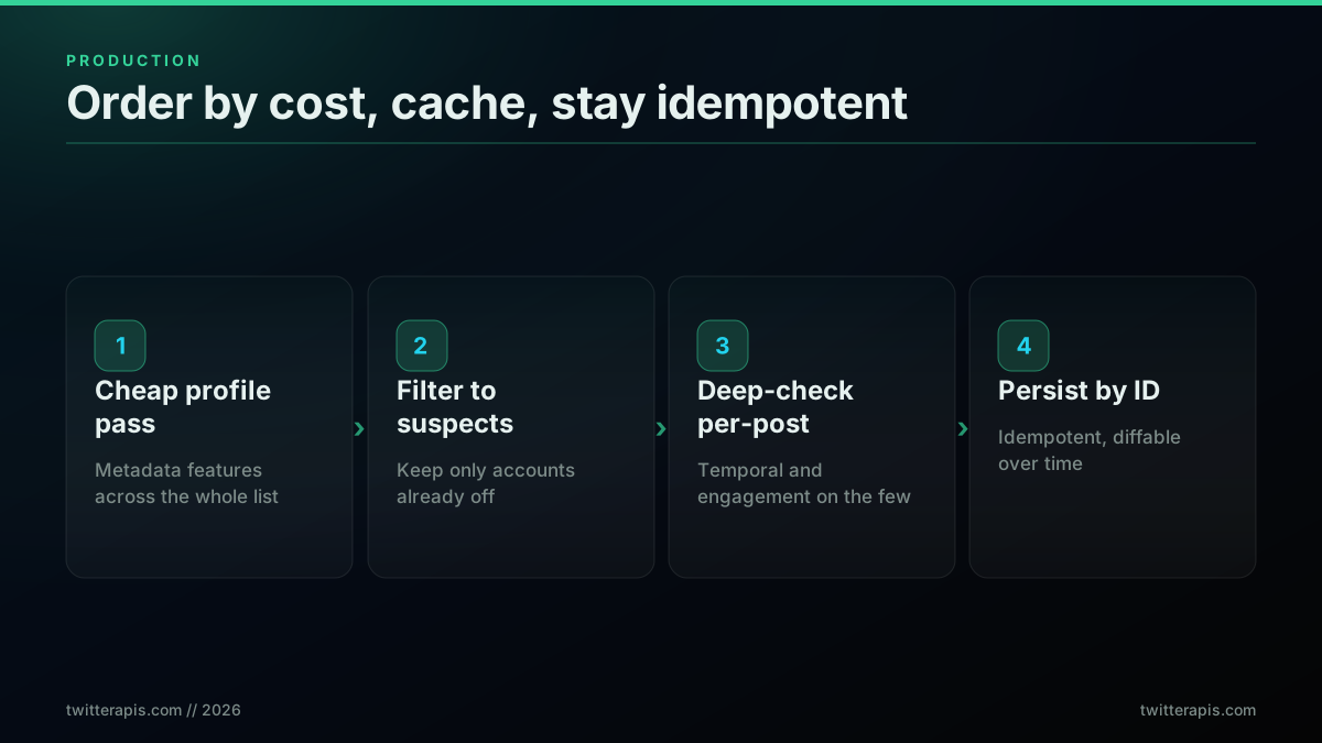
Order features by cost. The metadata features come off the profile object with no extra request. The temporal and engagement features cost per-post data. So run the cheap features across the entire list first, then spend per-post calls only on the accounts that already look suspicious. This cascade cuts the cost of a large scan by roughly an order of magnitude, because most of the list is cleared before any expensive call is made.

import time


def followers_page(handle: str, cursor: str | None = None) -> dict:
    # The endpoint ignores "count": page size is fixed at about 70 on the
    # first page and fewer after it, so page until the cursor runs out.
    params = {"userName": handle}
    if cursor:
        params["cursor"] = cursor
    resp = requests.get(f"{API_ROOT}/twitter/user/followers",
                        params=params, headers=AUTH, timeout=20)
    resp.raise_for_status()
    return resp.json()


def cheap_pass(handle: str, cap: int = 2000) -> dict:
    suspects, seen, cursor = [], 0, None
    while seen < cap:
        page = followers_page(handle, cursor)
        for f in page["followers"]:
            meta = metadata_features(f)
            points = 0
            if meta.posts_total > 5000 and meta.age_days < 90:
                points += 3
            if meta.log_follow_ratio > 1.1 and meta.following > 200:
                points += 2
            if meta.has_offplatform_link:
                points += 1
            if points >= 2:
                suspects.append({"userName": f["userName"], "cheap_points": points})
            seen += 1
        cursor = page.get("next_cursor")
        if not cursor:
            break
        time.sleep(0.5)   # respect the rate limit
    return {"checked": seen, "suspects": suspects,
            "bot_share_estimate": round(len(suspects) / max(seen, 1), 2)}

Cache and key by stable ID. Profile responses are worth caching across a run, since the same account often appears in multiple lists. And every result should be keyed by the account's numeric ID, not its handle, because handles change while IDs do not. Keying by ID makes the job idempotent, so a re-run does not double-count, and it lets you diff today's scan against last month's to watch whether an account's score is trending toward automation.

Deep-check incrementally. Feed the cheap-pass suspects into the full scorecard with per-post data, and re-score only the accounts whose cheap signals moved, rather than re-running the whole list every time. Incremental re-scoring is what makes a recurring audit cheap enough to run on a schedule.

The cost economics make this practical at real scale. A cheap pass reads only profile fields, so a two thousand account scan is a handful of calls; the deep check spends per-post calls only on the narrow suspect set. The Twitter API cost benchmark breaks down what large-list pulls actually cost, the export Twitter followers guide covers the pagination, and the best Twitter API for scraping comparison covers the read-access options that power the whole pipeline.

Where the off-the-shelf tools fit

None of this makes the existing tools worthless, and it is worth placing them honestly. Botometer is the name that comes up first, an academic project from Indiana University's Observatory on Social Media, which also publishes the BotometerLite dataset and research. You submit a handle and it returns a score. For a quick manual read on one account, it is genuinely useful.

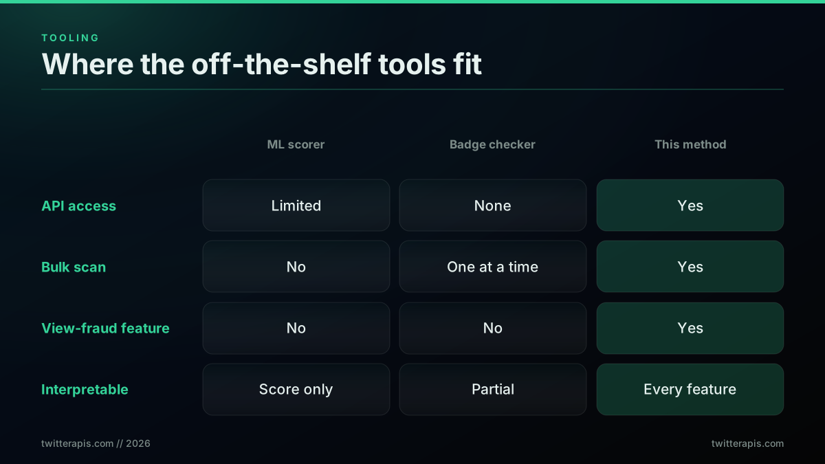
Its limits are structural rather than a knock on the work. It needs developer credentials to call, it predates the public view count so it cannot use the engagement-fraud family at all, and, per the MIT Sloan finding above, model-based detectors trained on one dataset generalize poorly to tactics they never saw. The web badge checkers sit at the other end: fast and setup-free, but one account at a time, with no API to wire into a pipeline. They give you a badge, not a feature.

The honest framing is that these tools are one more feature source, not a replacement for your own scoring. An off-the-shelf score can be a single input into the scorecard alongside the families you compute yourself. What no current tool gives you is programmatic access, bulk scanning, the engagement-fraud family, base-rate-aware evaluation, and an output you can read and tune. Those are the reasons to build the pipeline, and they are exactly the reasons this guide exists.

Getting the data: the fields these features need

Every feature above is computed from ordinary fields: creation date, follower and following counts, post count, per-post view, like, reply, and repost counts, and post timestamps. You need read access to profile and post data, and that is the whole dependency.

TwitterAPIs returns all of it as cleaned JSON from one Bearer-authenticated endpoint, which is what keeps each code sample to a few lines. If you are weighing providers first, the twitter API v2 vs TwitterAPIs breakdown covers the feature and cost differences, and the Apify scraper versus TwitterAPIs comparison places it against a marketplace scraper.

Step 1: Get a key. Sign up at /signup with an email and password. There is no developer-portal application and no card required. You start with 0.50 dollars in free credits, roughly 625 read calls or about 12,500 tweets, which is enough to build a labeled set and calibrate the score before you commit.

Step 2: Read a profile.

curl "https://api.twitterapis.com/twitter/user/info?userName=someaccount" \
  -H "Authorization: Bearer YOUR_KEY"

Step 3: Read recent posts with engagement fields.

curl "https://api.twitterapis.com/twitter/user/tweets?userName=someaccount&count=40" \
  -H "Authorization: Bearer YOUR_KEY"

From there the extractors run on the JSON directly. Read calls cost 0.0008 dollars each and return up to about twenty tweets per call, roughly 0.04 dollars per one thousand tweets, so scoring one account is a fraction of a cent and a two thousand follower cheap-pass scan is a few cents before any deep check. The API exposes 48 endpoints in total, 34 read endpoints plus 14 write endpoints; the simple write actions such as favorite, retweet, bookmark, follow, and media upload are also 0.0008 dollars per call, while tweet creation and DM send are 0.0016 dollars each, full-history reads are 0.0024 dollars, and full thread expansion is 0.0040 dollars. Write actions take a bring-your-own auth token and ct0 per request that are never stored. The twitter API cost guide and the cost calculator break the per-call economics down across monthly volumes, and the pricing page lists every tier.

The same detection logic runs against the official X API v2 if you want direct platform access; you pay more per call and configure field expansions, but the feature pipeline does not change. For that path, the how to get a twitter API key guide covers the developer portal end to end, and the rate limits reference covers the windows you will hit. For narrowing the post set you score when you are investigating a topic rather than an account, the advanced search operators guide is the reference, and the sentiment analysis walkthrough shows the content-analysis patterns that feed the language family.

Get Started

TwitterAPIs gives you 0.50 dollars in free credits at signup with no card required, enough to pull the profiles, timelines, and follower pages needed to build a labeled set and calibrate a score before committing. The links below map to each stage of the detection pipeline.

• Start free: Sign up for 0.50 dollars in credits, no card required
• Read profile and post fields: pricing at 0.0008 dollars per read call
• Estimate a scan's cost: cost calculator
• Pick a read-access provider: best Twitter API for scraping
• Pull post data without blocks: how to scrape tweets
• Audit a full follower list: export Twitter followers via API
• Feed the language family: Twitter sentiment analysis in Python
• Handle backoff on long scans: Twitter API rate-limit guide
• Read many histories at once: scrape tweet history via API
• Compare the full field: Twitter API alternatives

---

This guide describes detection features and thresholds for educational and analytical use. The engagement-ratio bands are presented as an illustrative working model that requires convergence across several features and calibration against labeled data, not as fixed constants or single-trigger verdicts. No specific account is named or characterized as automated. The MIT Sloan, Stanford Internet Observatory, Pew Research, and Ferrara references are cited for the general findings attributed to them. Thresholds should be tuned against a labeled set for your own use case. Method and pricing verified July 2026.