Twitter Trends API: Build Trending-Topic Detection by Location (2026)

There are two different questions hiding inside "get me Twitter trends," and answering the wrong one is why most builds go sideways. The first question is what is X showing right now for this place, and that is a fetch: pass a location code, read the ranked list back. The second is what is accelerating in this place, on my window, by my ranking rule, and that is a measurement problem you compute from raw tweets. This guide covers both, in that order, because the first one is a single call and most people who need it are being told to build the second.

Both routes run on one bearer token here. GET /twitter/trends and GET /twitter/trends/locations serve X's own trends-by-place list at approximately $0.0008 per call, with no developer application and no OAuth handshake. When the place you care about has no location code, which is most places, the second half of this guide builds a detection service from search: it scopes a query to any region, extracts candidate terms, scores them by velocity instead of raw volume, resists coordinated spam, keeps a rolling window of history, and serves the result from cache. Every snippet runs against a live endpoint, and every number in the cost math is a current per-call price.

TL;DR: For a place X already publishes trends for, call GET /twitter/trends?woeid=1 and you are done, at approximately $0.0008 per call against $0.010 per request on X's own API. Get the codes from GET /twitter/trends/locations, which returned 467 locations across 62 countries when measured on 2 August 2026, and cache it. For anywhere outside that list, compute trends from search: pull recent tweets for the place, extract hashtags and cashtags, and rank by acceleration rather than raw count. Score with a velocity or z-score signal, count distinct authors to blunt bots, keep two windows so you can measure change, and cache the ranked list between polls. A fifteen-minute single-region search-derived tracker costs roughly $2.30 a month. The engine below is a few hundred lines of Python.

import re
import requests
from collections import Counter

BASE = "https://api.twitterapis.com/twitter"          # one per-call read endpoint
TAG_RE = re.compile(r"(?:#\w+|\$[A-Za-z]\w*)")         # hashtags and alphabetic cashtags

def top_tags(query, api_key, n=10):
    r = requests.get(f"{BASE}/tweet/advanced_search",
                     params={"query": query, "product": "Latest"},
                     headers={"Authorization": f"Bearer {api_key}"}, timeout=10)
    r.raise_for_status()
    votes = Counter()
    for tweet in r.json().get("tweets", []):
        for tag in {m.lower() for m in TAG_RE.findall(tweet.get("text", ""))}:
            votes[tag] += 1        # one vote per tweet, deduped inside the tweet
    return votes.most_common(n)

for tag, hits in top_tags("(Chicago OR #Chicago) lang:en", "YOUR_API_KEY"):
    print(f"{tag:<18} {hits}")

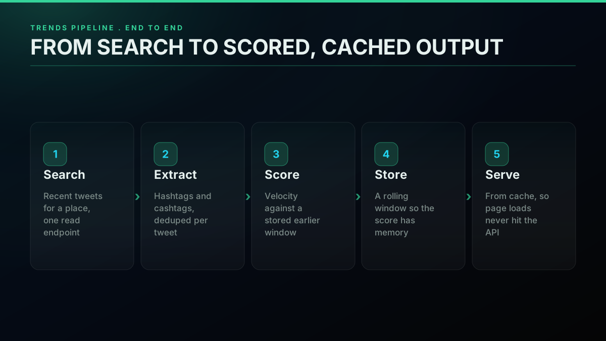
That is a working trend counter in fewer than twenty lines. It pulls the newest tweets for a place, extracts hashtags and cashtags with a single regular expression, and ranks by how many distinct tweets each tag appears in. Everything below turns this into a system: geo queries that actually isolate a region, a velocity score so you surface what is climbing rather than what is merely large, an author-based spam filter, a windowed store so the score has memory, and a cost model so you can size the bill before you deploy.

Before any of that, though, check whether you need it at all.

Route one: ask for the list X is already publishing

If your target is a country or a major city, X computes a trend list for it and you can just read it. One call, one parameter.

curl "https://api.twitterapis.com/twitter/trends?woeid=1&count=3" \
  -H "Authorization: Bearer $TWITTERAPIS_KEY"

Run live on 2 August 2026, that returns:

{
  "location": { "name": "Worldwide", "woeid": 1 },
  "as_of": "2026-08-02T16:55:59Z",
  "created_at": "2026-08-01T04:07:08Z",
  "count": 3,
  "trends": [
    { "name": "PSD MOGULARRIVAL FS26", "query": "%22PSD+MOGULARRIVAL+FS26%22",
      "tweet_volume": null, "is_hashtag": false, "rank": 1 },
    { "name": "#日向坂で会いましょう", "query": "...",
      "tweet_volume": null, "is_hashtag": true, "rank": 2 },
    { "name": "#VIVANT", "query": "%23VIVANT", "tweet_volume": null,
      "is_hashtag": true, "rank": 3 }
  ]
}

Four things in that response are worth reading properly rather than skipping.

rank is the position X served, not a score you computed. The list arrives in trending-rank order and the field is assigned before any count truncation, so it stays stable whether you ask for three trends or fifty.

query is pre-encoded and name is not. Use query to build a search URL and name for display. Building a search from name will break on the first hashtag with a non-ASCII character in it, which as the response above shows is roughly immediately.

tweet_volume is often null, and that is X's behaviour rather than a gap. X reports a volume for some trends and not others. Treat null as unknown, never as zero, or a ranking that multiplies by volume will silently bury every trend X declined to size.

as_of and created_at are different clocks, and the gap is larger than people expect. as_of is when the list was served to you. created_at is X's own stamp for when it computed the list. On the call above, as_of was 2 August at 16

UTC and created_at was 1 August at 04 UTC, a gap of roughly thirty-seven hours. A United States call in the same session reported a gap of roughly twenty hours. If your product implies the list is live to the second, read created_at and say what it says instead. A per-minute poll against this endpoint will not make X's list any fresher than X computed it.

There is also a response cache in front of this, keyed on the exact parameter set, with a sixty-second default lifetime. Two identical back-to-back calls in the same session returned a byte-identical as_of of 2026-08-02T16:58:17Z, which is the cache doing its job. Changing count changes the key, so it is a different cache entry.

Finding the WOEID, and what the table actually covers

GET /twitter/trends/locations returns every location X publishes a trend list for. Call it once and cache it: the list changes on the order of months, and the endpoint exists so you never have to hardcode a code table.

import requests

BASE = "https://api.twitterapis.com/twitter"
H = {"Authorization": f"Bearer {API_KEY}"}

def woeid_for(place_name):
    r = requests.get(f"{BASE}/trends/locations", headers=H, timeout=30)
    r.raise_for_status()
    for loc in r.json()["locations"]:
        if loc["name"].lower() == place_name.lower():
            return loc["woeid"]
    return None

def trends(woeid=1, count=50):
    r = requests.get(f"{BASE}/trends", params={"woeid": woeid, "count": count},
                     headers=H, timeout=30)
    r.raise_for_status()
    return r.json()

print(woeid_for("Chicago"))          # -> 2379574

Measured against a live call on 2 August 2026, the list holds 467 locations: 1 Supername (Worldwide, WOEID 1), 62 countries, 402 towns and cities, and 2 that X reports with no place type. Sixty-four of those locations are in the United States, from Albuquerque and Atlanta through to the smaller metros.

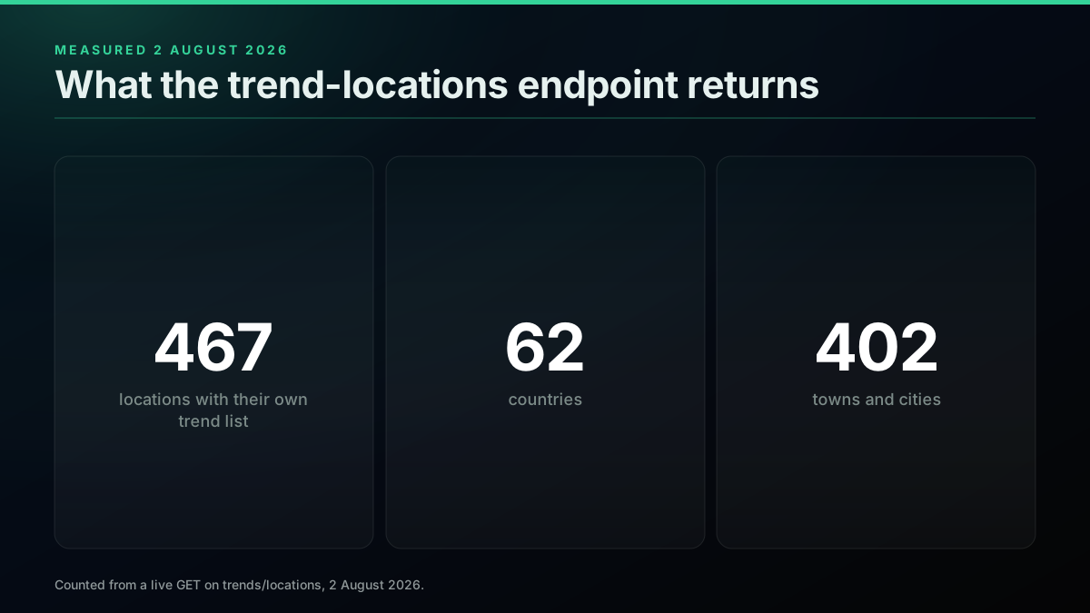
What the location table actually covers, counted from a live call

That is the honest size of the direct route, and it is the number that decides which half of this guide you need. Four hundred and sixty-seven places is a lot if you want national or big-metro trends. It is nothing if you want a neighbourhood, a mid-size town, or a topic rather than a place. There is no code for those and no endpoint can invent one.

If you would rather not do the lookup at all, pass a country name and let the API resolve it server-side:

curl "https://api.twitterapis.com/twitter/trends?country=United%20States&count=3" \
  -H "Authorization: Bearer $TWITTERAPIS_KEY"
# -> {"location":{"name":"United States","woeid":23424977}, ...}

A name the table does not contain fails loudly rather than quietly. ?country=Zzqnotarealcountry returns HTTP 400 with "No trends location matched that country. Use /twitter/trends/locations for the supported set." That matters more than it sounds: an empty trends array would be indistinguishable from a real quiet period, and you would ship a dashboard that shows nothing and reports no error.

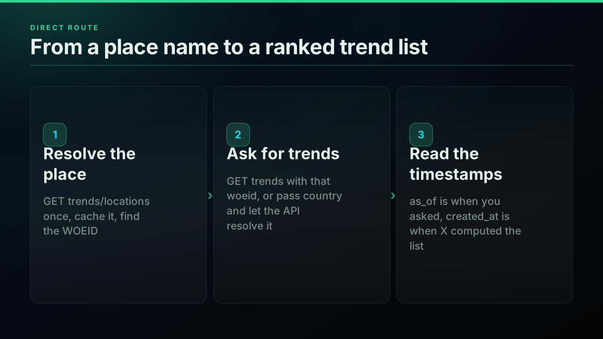
The direct route is three steps, and the third one is the one that keeps your freshness claim honest

What the direct route costs

Both trends endpoints are billed as standard reads at approximately $0.0008 per call. X's own API prices the same operation on its published rate card, which confirms pay-per-usage with no subscriptions, and its Trends row is $0.010 per request.

Poll cadence	Calls per month	At approximately $0.0008	At X's $0.010
Hourly, one location	720	approximately $0.58	$7.20
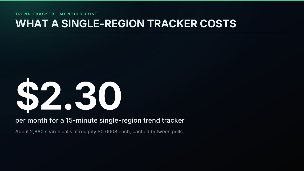
Every 15 minutes, one location	2,880	approximately $2.30	$28.80
Every 5 minutes, one location	8,640	approximately $6.91	$86.40
Every 15 minutes, 10 locations	28,800	approximately $23.04	$288.00

The sixty-second response cache means a poll faster than once a minute buys you repeated bytes rather than fresher data, and given the created_at gap above, a poll faster than a few minutes is buying you very little regardless. Pick the slowest cadence your product tolerates and spend the savings on covering more locations.

The rest of this guide is the other route: what to do when the WOEID table has no code for the place you care about.

What a Twitter trend actually is

A trend is a rate, not a total. A hashtag that has sat at a steady two hundred mentions all week is popular, but it is not trending. A tag that went from four mentions to eighty in the last twenty minutes is trending even though its total is smaller. The whole job of a trends pipeline is to measure that change over a defined window and rank by it, which means a trend only exists relative to a clock and a place you choose.

This reframing matters because it explains what the trends endpoint can and cannot tell you. It returns a ranked list, and the ranking is a black box. Nobody outside the company knows the exact window it uses, how heavily it personalizes, or how it filters promoted and spam content, and the response carries no score, only a position. When you compute trends from search you own every one of those knobs: the length of the window, the minimum count a tag needs to qualify, how aggressively you discount repeat authors, and whether a cashtag counts the same as a hashtag. For a product that has to explain its rankings to a user or a reviewer, a pipeline you can describe line by line beats a list you cannot audit, even when the list is one cheap call away.

The tradeoff is real. Computing a trend is more work than reading one, and the quality of your output depends entirely on the sample you pull and the score you apply. The rest of this guide is about making both good. If you want the request-and-response basics the code assumes, the complete 2026 Twitter API tutorial covers the fetch model, and the Python Twitter API tutorial builds the HTTP layer from the ground up.

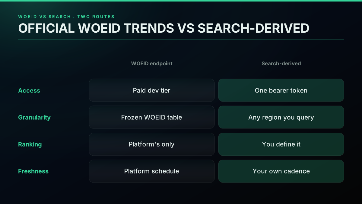
Route two: when the trends endpoint cannot answer your question

Route one is the right answer for a country or a big metro. Three walls push builders off it for everything else, and they are worth naming precisely because two of them are not about price.

The first wall is coverage, and it is the one that decides most builds. Four hundred and sixty-seven locations is the whole table. If you are building for a neighbourhood, a mid-size town, a university, an industry, or any topic that is not a place at all, there is no code for it and there never will be, because the WOEID scheme is a frozen artifact rather than a growing index. No API in front of X can invent an entry.

The second wall is rigidity. Where a code does exist, you get X's definition of a trend and nothing else. You cannot change the window, the ranking rule, the minimum count, or the spam filter, and you cannot see any of them either. For a product that has to explain a ranking to a user or a reviewer, an unauditable list is a liability regardless of how cheap the call is.

The third wall is freshness, which the measurement in route one already showed: the created_at on a live worldwide list read roughly thirty-seven hours older than the call that fetched it. That is fine for a widget and useless for a breaking-news product that needs a minute-level pulse.

Access is a fourth wall on X's own API specifically, though not on this one. Reading trends there requires a developer account with a funded balance, and the 2026 X API pricing change breakdown tracks how the read model shifted, with the is the Twitter API free explainer laying out what the free tier will and will not return. You can confirm the current rates on the official X API pricing page and cross-check the read model against the X developer documentation.

Developers have been blunt about how the read paywall feels once it lands on a hobby project or a small tool. Here is one builder recalculating a bot after the free tier vanished:

https://x.com/cmcwain/status/2062052786838421622

And another walking away from the platform entirely once the per-post read price showed up:

https://x.com/Tunables/status/2062529533215928355

The same frustration is a recurring thread among web developers weighing whether the official plans are worth it at all:

Twitter API plans are a joke from r/webdev

The search-derived route clears the first three walls. You pull tweets from a read endpoint you can reach on a bearer token, you define the window and the ranking, and you set the cadence. A builder in March 2026 described exactly this build and what it cost him to run:

The hardest thing growing on X is staying ahead of trending topics. It can easily turn into a full time job. So I built a trend radar with OpenClaw that helps me snipe trends as they form. The whole setup costs me $2 per month in API calls.

— @leonabboud view on X

Two dollars a month is the right order of magnitude, and it matches the cost table further down almost exactly. If you are coming off the official API, the Twitter API v2 versus TwitterAPIs guide is the translation table, the key walkthrough covers signup to first call, and the migration guide walks a real switch.

WOEID versus semantic geo: two ways to say "here"

There are two ways to tell an API where you mean, and they behave very differently. The WOEID way hands the platform a numeric code and reads back the list X built for it. The semantic way describes the place in words inside your search query and lets the text do the scoping. Neither one wins outright. The code is more accurate wherever it exists, because it is X's own answer rather than your approximation of it. Words are the only option everywhere else, which turns out to be most places.

WOEID, short for Where On Earth ID, comes from an old geolocation service, and the global trends list lives under the code 1. Chicago is 2379574, London is 44418, the United States is 23424977, all confirmed live from trends/locations on 2 August 2026. The scheme's problem is not accuracy, it is reach: 467 entries against the world's cities, and a frozen table that never grows. The WOEID reference documents the history if you want it. The practical takeaway is that a code-based system caps the granularity of your product at whatever the table happens to include, which is a hard ceiling you did not choose. Check the table first. If your place is on it, take the code and skip the rest of this guide. If it is not, keep reading.

The community around this problem is mostly people who checked and found no code. A developer building a location-scoped trends viewer hit exactly that shape and shipped it as a custom app rather than a wrapper over the official list:

the r/reactjs thread, at roughly 282 upvotes and 32 comments, where a developer ships a Twitter trends app for viewing trending topics and hashtags from a specific location from r/reactjs

Semantic geo trades that ceiling for a tuning problem. You describe a place with a bundle of terms and accept that the bundle is fuzzy, then sharpen it. The advanced search operators reference lists every operator you can combine, and the pattern below turns a place into a query fragment.

from dataclasses import dataclass, field

@dataclass
class Place:
    name: str
    aliases: list[str] = field(default_factory=list)   # abbreviations, hashtags, landmarks
    lang: str = "en"

    def as_query(self, topic: str = "") -> str:
        terms = [self.name, *self.aliases]
        where = "(" + " OR ".join(dict.fromkeys(terms)) + ")"   # dedupe, keep order
        parts = [p for p in (topic, where, f"lang:{self.lang}") if p]
        return " ".join(parts)

chicago = Place("Chicago", ["#Chicago", "CHI", "Chi-town", "Loop"])
print(chicago.as_query())
# -> (Chicago OR #Chicago OR CHI OR Chi-town OR Loop) lang:en

The bundle is where precision lives. Add the local language to the filter when a region is not primarily English. Include the short form locals actually tag with, since a city hashtag often beats the full name in volume. Add a landmark or two that rarely appear outside the area to anchor ambiguous names. The goal is a query where most of the tweets you pull genuinely concern the place, because every off-topic tweet dilutes the ranking downstream. Tune the breadth against the sample size: too narrow and you have no signal, too broad and the local trend blurs into the national one.

Authentication and your first search call

Authentication on a per-call read API is a single header, not an OAuth handshake. It is the same header the two trends endpoints in route one used, and the same one every snippet below uses. There is no app review, no elevated-access form, and no token refresh loop. You pass a bearer token on every request and you are reading tweets in about thirty seconds after signup. That is the whole ceremony.

curl "https://api.twitterapis.com/twitter/tweet/advanced_search?query=%28Chicago%20OR%20%23Chicago%29%20lang%3Aen&product=Latest" \
  -H "Authorization: Bearer YOUR_API_KEY"

That request returns the newest tweets matching the query as JSON. If you are switching from the official API, the only real change is the base URL and the auth header; the tweet fields you parse are the same shape. Grab a key on the sign up page, and if you want to see what your spend will look like before writing a line, the cost calculator models it. Below is the same call in Python, wrapped so the rest of the engine has one place to make a request.

import requests

class Client:
    def __init__(self, api_key, base=BASE, timeout=10):
        self.session = requests.Session()
        self.session.headers["Authorization"] = f"Bearer {api_key}"
        self.base = base
        self.timeout = timeout

    def search(self, query, query_type="Latest"):
        r = self.session.get(f"{self.base}/tweet/advanced_search",
                             params={"query": query, "product": query_type},
                             timeout=self.timeout)
        r.raise_for_status()
        return r.json().get("tweets", [])

A single Session reuses the underlying connection across polls, which matters once you are calling the endpoint every fifteen minutes for weeks. The raise_for_status call surfaces a bad response as an exception you will catch in the retry layer later. The Requests library documents both behaviors, and the best practices guide covers connection reuse and timeout tuning in depth.

Reading the tweet object: the fields a trend pipeline needs

A trends pipeline touches only a few fields on each tweet, so it pays to know which ones and to read them defensively. A search response returns a list of tweet objects, and four fields drive detection: the text, the author identifier, the creation timestamp, and the tweet identifier. The text feeds tag extraction, the author identifier feeds the spam filters, the timestamp lets you weight recent tweets and bucket by window, and the identifier lets you dedupe across pages so one tweet never votes twice.

Reading defensively matters because field names drift and optional fields go missing. An account deleted between the tweet and your fetch can leave the author block null, a retweet can nest the original text one level down, and a truncated field can hide part of the tag set. The reader below pulls each field with a fallback and skips a tweet that has no usable text rather than letting a missing value crash the loop.

from datetime import datetime

def read_tweet(raw):
    text = raw.get("text") or raw.get("full_text") or ""
    author = (raw.get("author") or {}).get("id") or raw.get("authorId")
    tid = raw.get("id") or raw.get("id_str")
    created = raw.get("created_at")
    ts = None
    if created:
        try:
            ts = datetime.strptime(created, "%a %b %d %H:%M:%S %z %Y")
        except ValueError:
            ts = None
    return {"id": tid, "author": author, "text": text, "ts": ts}

def usable(tweets):
    for raw in tweets:
        t = read_tweet(raw)
        if t["text"] and t["id"]:
            yield t

Deduping is the other reason to read the identifier. When you walk several cursor pages to build a larger sample, the pages can overlap, and a tweet that appears on two pages would otherwise vote twice. Keep a set of seen identifiers across the whole refresh and skip a tweet you have already counted. That same set doubles as your page-walk terminator: when a page adds no new identifiers, you have reached the end of fresh results and can stop paging. The rate limits guide covers how to pace those paged calls, and the best practices guide covers cursor handling.

def collect(client, query, max_pages=5):
    seen, batch = set(), []
    for _ in range(max_pages):
        page = client.search(query)          # a real client walks the cursor here
        fresh = [t for t in usable(page) if t["id"] not in seen]
        if not fresh:
            break                            # no new tweets: stop paging
        seen.update(t["id"] for t in fresh)
        batch.extend(fresh)
    return batch

Extracting candidates: hashtags, cashtags, and phrases

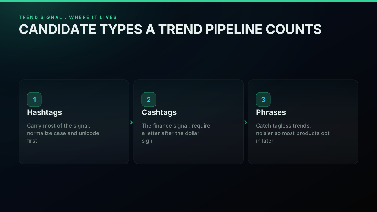
A candidate is any token that could become a trend. Hashtags carry most of the signal, cashtags carry the finance signal, and multi-word phrases catch the trends that never get a tag at all. The extraction step turns a batch of raw tweet text into a bag of these candidates, deduped within each tweet so one tweet votes once no matter how many times it repeats a tag.

import re
from collections import Counter

TAG_RE = re.compile(r"#\w+|\$[A-Za-z]\w*")     # #hashtag or $CASHTAG (letter after $)
WORD_RE = re.compile(r"[A-Za-z][A-Za-z']+")    # plain words for phrase candidates

def candidates(text, phrases=False, phrase_len=2):
    tags = {m.lower() for m in TAG_RE.findall(text)}
    if not phrases:
        return tags
    words = [w.lower() for w in WORD_RE.findall(text)]
    grams = {" ".join(words[i:i + phrase_len])
             for i in range(len(words) - phrase_len + 1)}
    return tags | grams

def tally(tweets, **kw):
    counts = Counter()
    for tweet in tweets:
        for c in candidates(tweet.get("text", ""), **kw):
            counts[c] += 1        # distinct-tweet count, spam-resistant by design
    return counts

The cashtag rule requires a letter right after the dollar sign, so a price like $7,000 never pollutes the ranking while $NVDA still counts. The optional phrase mode adds every two-word n-gram, which surfaces emerging topics that people discuss without a tag. Phrases are noisier, so most products start with tags only and turn phrases on for a specific analysis. If you want to layer meaning on top of the same batch, the Twitter sentiment analysis tutorial scores tone over the exact tweets you already pulled.

Normalizing tags before you count them

Two tags that look the same to a human can look different to a counter, which quietly splits a trend across variants and weakens its rank. #WorldCup, #worldcup, and a fullwidth-character copy are three keys unless you normalize first. Lowercasing is the baseline, and the extractor above already does it. Two more steps help: strip trailing punctuation that sneaks into a token, and fold unicode look-alikes so an accented or fullwidth variant collapses onto its plain form.

import unicodedata

def normalize_tag(tag):
    tag = unicodedata.normalize("NFKC", tag)     # fold fullwidth/compatibility forms
    return tag.strip(".,!?;:'\"()[]").lower()

Near-duplicate folding is a judgment call. Collapsing #WorldCup2026 into #WorldCup merges a specific tag into a general one, which you may or may not want. A safe default is to normalize only the mechanical differences, casing, punctuation, and unicode form, and to leave semantically distinct tags separate. Over-aggressive folding hides real sub-trends; under-normalizing splits one trend into several weak ones. Start conservative and widen only when you watch the same trend fragment across obvious variants.

One tweet batch rarely holds enough tweets for a stable count, so you walk the search cursor until the sample is large enough to rank confidently. The how to scrape tweets walkthrough covers the cursor pattern, and the rate limits guide explains how to pace those paged calls so a tight loop does not trip a limit. This short screencast on getting trend context out of tweet data mirrors the extract-and-count loop you just wrote:

https://www.youtube.com/watch?v=cT_r7LRDAiw

Scoring: from raw counts to velocity and z-scores

Raw counts answer the wrong question. Sorting by count surfaces the tags that are always big, which is exactly what you do not want. The fix is to score each tag by how much its current count deviates from what it usually does, so a tag climbing fast rises even when its total is modest. There are two scores worth knowing, and they suit different products.

The first is a simple velocity, the change over a window relative to the earlier count. It is cheap and intuitive.

def velocity(current, previous, top_n=10):
    """Rank by fractional change: how much faster a tag appears now vs before."""
    scored = {}
    for tag, now in current.items():
        before = previous.get(tag, 0)
        scored[tag] = (now - before) / (before + 1)   # +1 keeps new tags finite
    return sorted(scored.items(), key=lambda kv: kv[1], reverse=True)[:top_n]

Velocity has a weakness: a tag that jumps from zero to three has a huge fractional change but is almost certainly noise. So gate it with a floor. Require a minimum current count before a tag is even eligible to rank, which removes the long tail of one-off spikes that would otherwise dominate.

def ranked(current, previous, min_count=8, top_n=10):
    eligible = {t: n for t, n in current.items() if n >= min_count}
    return velocity(eligible, previous, top_n=top_n)

The second score is a z-score, which is worth the extra bookkeeping when you track a tag over many windows rather than just two. Instead of comparing now against one earlier window, you compare now against the tag's own recent average and spread. A z-score of three means the tag is three standard deviations above its normal rate, a much stronger claim than a raw jump. The standard score reference has the formula; the code keeps a short history per tag and computes it directly.

import statistics

def z_scores(history, current, min_history=5, top_n=10):
    """history: dict[tag] -> list of past window counts. current: dict[tag] -> count."""
    scored = {}
    for tag, now in current.items():
        past = history.get(tag, [])
        if len(past) < min_history:
            continue
        mu = statistics.fmean(past)
        sigma = statistics.pstdev(past) or 1.0     # avoid divide-by-zero on flat tags
        scored[tag] = (now - mu) / sigma
    return sorted(scored.items(), key=lambda kv: kv[1], reverse=True)[:top_n]

For a smoother baseline that reacts to recent windows without a hard cutoff, an exponentially weighted moving average is a good middle ground: it weights recent counts more heavily and needs only one number in storage per tag rather than a full list. The exponential smoothing reference covers the weighting; in practice you keep a running mean, blend each new count in with a small alpha, and score the deviation from that running mean. Whichever score you pick, the shape of the pipeline is the same: pull, extract, compare against stored history, rank.

Tumbling versus sliding windows

The window is the interval your score compares across, and there are two ways to shape it. A tumbling window advances in fixed, non-overlapping steps: every fifteen minutes you take a fresh snapshot and compare it to the last one. A sliding window moves continuously, always comparing the most recent interval to the one before it, which smooths the score at the cost of more bookkeeping. Most trends products start tumbling because it maps cleanly onto a poll loop: one poll, one snapshot, one comparison.

The window length is a tradeoff between reactivity and stability. A short window of five minutes reacts fast and catches breaking spikes, but it is noisy, and a quiet stretch can make everything look like it is moving. A long window of an hour is stable and calm, and it can miss a spike that peaks and fades between snapshots. Pick the window from the product: a breaking-news feed wants short windows and tolerates noise, a daily digest wants long windows and rejects it.

from collections import deque

def sliding_deltas(snapshots, top_n=10):
    """snapshots: deque of (ts, {tag: count}); compare newest to prior."""
    if len(snapshots) < 2:
        return []
    (t1, prev), (t2, cur) = snapshots[-2], snapshots[-1]
    span = max(1.0, t2 - t1)                       # real elapsed seconds
    rate = {tag: (cur.get(tag, 0) - prev.get(tag, 0)) / span for tag in cur}
    return sorted(rate.items(), key=lambda kv: kv[1], reverse=True)[:top_n]

The subtle part is aligning the window to the poll. If your window is fifteen minutes but a poll occasionally takes two minutes to walk its pages, the effective interval drifts. Timestamp each snapshot when you store it, as the window store already does, and compute the real elapsed time between the two snapshots you compare rather than assuming a clean interval. A velocity divided by the actual elapsed seconds stays comparable across polls even when the polls themselves run uneven.

Spam and coordination resistance

A trend score is only as trustworthy as the accounts behind it. A coordinated push, whether a paid campaign or a bot ring, can inflate a tag by having many accounts repeat it, and a naive tweet count rewards exactly that behavior. The single most effective defense costs nothing extra: count distinct authors per tag instead of distinct tweets. A tag then has to earn its rank from a broad base rather than a loud few, and the tweets are ones you already fetched.

def author_spread(tweets, stop_tags=frozenset(), top_n=10):
    seen = {}   # tag -> set of author ids
    for tweet in tweets:
        author = (tweet.get("author") or {}).get("id") or tweet.get("authorId")
        for tag in {m.lower() for m in TAG_RE.findall(tweet.get("text", ""))}:
            if tag in stop_tags:
                continue
            seen.setdefault(tag, set()).add(author)
    ranked = sorted(seen.items(), key=lambda kv: len(kv[1]), reverse=True)
    return [(tag, len(authors)) for tag, authors in ranked[:top_n]]

For a sharper filter, measure how evenly the authors are distributed. If ninety percent of a tag's tweets come from three accounts, its author distribution has low entropy and the tag is suspect even if the distinct-author count looks fine. Shannon entropy over the per-author tweet counts gives you a single number: high entropy means a broad, organic base, low entropy means concentration. The entropy reference has the math, MathWorld's Shannon entropy writeup walks through the same formula with worked examples, and a per-tag guard is short.

import math

def author_entropy(author_counts):
    """author_counts: list of tweet counts per author for one tag."""
    total = sum(author_counts)
    if total == 0:
        return 0.0
    return -sum((c / total) * math.log2(c / total) for c in author_counts if c)

def looks_organic(author_counts, floor=1.5):
    return author_entropy(author_counts) >= floor

Add a small stopword set for tags that are perennially present in your niche and carry no news value, the equivalent of dropping "the" from a word count. Between the author-spread rank, the entropy guard, the count floor, and the stopword set, you have four cheap filters that separate a genuine emerging topic from an inflated one. If you want to go further and actually score how bot-like the accounts are, the bot detection guide covers the signals you can compute from the same batch.

Storing rolling windows: the state problem

Every score above needs memory. Velocity needs the previous window, a z-score needs a short history, an EWMA needs a running mean. So the pipeline has to keep a little state between polls, and where you keep it decides how far the system scales. For one region, a couple of in-process dictionaries are enough. For many regions polled continuously, you want a store that survives a restart and can be read by more than one process. SQLite is the simplest option that satisfies both, since it ships as a single file with no server to run.

import sqlite3, json, time

class WindowStore:
    """Keeps the last K count-snapshots per region in SQLite."""
    def __init__(self, path="trends.db", keep=6):
        self.db = sqlite3.connect(path)
        self.keep = keep
        self.db.execute("""CREATE TABLE IF NOT EXISTS windows
            (region TEXT, ts REAL, counts TEXT)""")
        self.db.commit()

    def push(self, region, counts):
        self.db.execute("INSERT INTO windows VALUES (?,?,?)",
                        (region, time.time(), json.dumps(counts)))
        # trim to the most recent `keep` snapshots for this region
        self.db.execute("""DELETE FROM windows WHERE region=? AND ts NOT IN
            (SELECT ts FROM windows WHERE region=? ORDER BY ts DESC LIMIT ?)""",
            (region, region, self.keep))
        self.db.commit()

    def history(self, region):
        rows = self.db.execute(
            "SELECT counts FROM windows WHERE region=? ORDER BY ts", (region,)).fetchall()
        return [json.loads(r[0]) for r in rows]

The sqlite3 module ships with Python, so a single-file store needs no infrastructure and survives a restart, which an in-memory dict does not. The keep parameter caps how many windows you retain per region, which bounds both the disk footprint and the history a z-score can look back over. Rebuilding the per-tag history for scoring is then a matter of transposing those snapshots.

def history_by_tag(snapshots):
    """Turn a list of {tag: count} snapshots into {tag: [counts over time]}."""
    by_tag = {}
    for snap in snapshots:
        for tag, count in snap.items():
            by_tag.setdefault(tag, []).append(count)
    return by_tag

Once you are tracking many regions and want more than one worker to read the ranked list, promote the store to Redis with a time-to-live per region so a stale entry expires on its own if a poll ever fails. The Redis key-expiration docs describe the TTL behavior you would lean on. The pattern is the same either way: write the snapshot on each poll, read the history when you score.

The cold-start problem: ranking before you have history

Every score above needs a previous window, so the first poll of a new region has nothing to compare against and the velocity is undefined. If you ship the naive version, a brand-new region returns an empty or garbage list until the second poll lands, which is a visible bug on any freshly added location. There are two clean ways to handle the cold start.

The first is to fall back to raw counts on the first poll and switch to velocity once a baseline exists. The ranked list is less meaningful on the very first refresh, but it is populated and reasonable, and it self-corrects on the next interval. The second is to warm the baseline immediately by pulling a slightly older sample with a time filter that fetches tweets from the prior interval, so you hold both windows after a single startup burst rather than waiting a full interval.

def first_or_velocity(current, history, min_count=8, top_n=10):
    if not history:                                # cold start: no baseline yet
        counts = {t: n for t, n in current.items() if n >= min_count}
        return sorted(counts.items(), key=lambda kv: kv[1], reverse=True)[:top_n]
    return ranked(current, history[-1], min_count=min_count, top_n=top_n)

Which one you pick depends on how much the first interval matters. A dashboard a user is watching wants the warm-baseline approach so it looks correct immediately. A background feed that nobody sees for the first fifteen minutes can take the simpler raw-count fallback and let the second poll fix it. Either way, make the first poll a defined case rather than an accidental empty list, because an empty list on a new region is the kind of bug that ships unnoticed and surfaces in a demo.

Polling cadence and the cost math

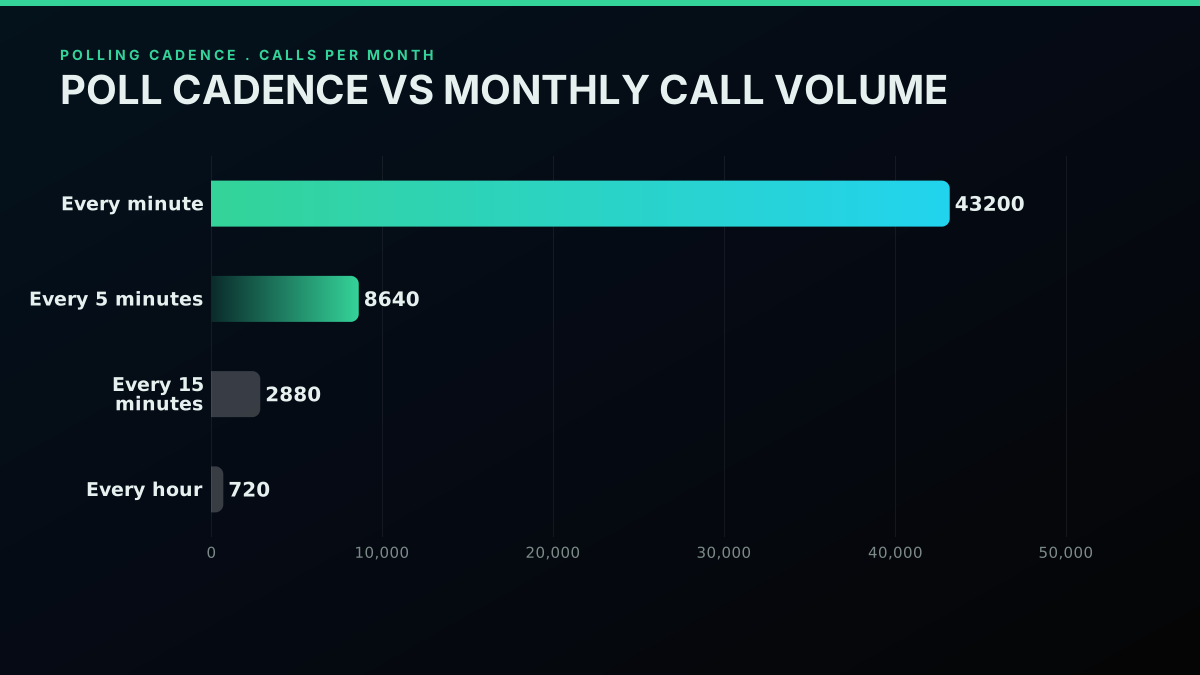
Cadence is the one lever that sets both your freshness and your bill, because every refresh is one or more search calls. Sizing it is simple arithmetic once you know the per-call rate. On a per-call read API the standard rate is approximately $0.0008 per call, one call returns roughly twenty tweets, and that works out to approximately $0.04 per 1,000 tweets. Signup includes approximately $0.50 in free credits, enough for around 625 calls with no card required. The pricing page is the source of truth, and the Twitter API cost breakdown compares per-call against the official tiers across realistic scenarios.

Here is what cadence does to a single region, at one search call per refresh:

Refresh interval	Calls per month	Approx cost per month
Every minute	43,200	approximately $34.56
Every 5 minutes	8,640	approximately $6.91
Every 15 minutes	2,880	approximately $2.30
Every hour	720	approximately $0.58

The every-minute row costs roughly sixty times the hourly row for the same region, and unless you are tracking breaking news the coverage difference rarely justifies it. Two more factors move the real bill. If you walk several cursor pages per refresh to get a bigger sample, multiply the call count by the pages. If you serve many regions, the calls scale linearly with region count. A three-region tracker polling every fifteen minutes at one page each is close to 8,640 calls a month, or roughly $6.91 before caching. The cheapest Twitter API comparison and the cost benchmark put those numbers next to other providers.

Sizing the sample: how many pages per poll

One search page rarely holds enough tweets to rank confidently, so the real question is how many pages to walk per poll, and that choice moves both your accuracy and your bill. A larger sample stabilizes the ranking because a tag's count stops swinging on the luck of which tweets a single page returned, but each extra page is another call. The tradeoff is concrete: if one page returns roughly twenty tweets and you want a two-hundred-tweet sample for a stable count, that is ten pages, and ten pages per poll multiplies your call count and cost by ten.

Size the sample from the region's volume rather than a fixed page count. A busy metro produces enough tweets in a fifteen-minute window that two or three pages give a stable ranking, while a quiet region may need more pages to gather the same count, or may simply not have enough recent tweets to rank at all. A good heuristic is to page until either the sample crosses a target size or a page returns no new identifiers, whichever comes first, which the collect helper above already does. That caps the cost on quiet regions and gathers a deep enough sample on busy ones without a hardcoded page count that is wrong for both.

Caching is what keeps this cheap under real traffic. The poll worker refreshes the ranked list on the cadence you chose, and the web tier reads that cached list on every page load without ever calling the API. Your spend then tracks the poll schedule, not your visitor count, which is the entire reason a real-time trends feature can cost a few dollars a month.

import time

def poll_loop(engine, region, interval=900):
    """Refresh one region on a fixed cadence; the app reads engine.cache[region]."""
    while True:
        try:
            engine.refresh(region)     # fetch, score, write to cache + WindowStore
        except Exception as exc:       # never let one bad poll kill the loop
            engine.log_error(region, exc)
        time.sleep(interval)

A worked build: a multi-region trends service

Wiring the pieces together gives a small service that powers a "what is trending near you" feature. It holds a set of regions, refreshes each on a schedule into a cache and the window store, scores the newest snapshot against the stored history, and serves the ranked list from cache on every request. The engine below reuses the Client, tally, ranked, and WindowStore from earlier sections.

class TrendEngine:
    def __init__(self, client, store, regions):
        self.client = client
        self.store = store
        self.regions = regions          # dict[name] -> Place
        self.cache = {}                  # name -> ranked list, read by the web tier

    def refresh(self, name):
        place = self.regions[name]
        tweets = self.client.search(place.as_query())
        current = dict(tally(tweets))                    # {tag: distinct-tweet count}
        history = self.store.history(name)
        previous = history[-1] if history else {}
        self.cache[name] = ranked(current, previous)     # velocity + count floor
        self.store.push(name, current)                   # roll the window forward

    def trending(self, name):
        return self.cache.get(name, [])

    def log_error(self, name, exc):
        print(f"[trend] {name}: {exc}")

regions = {
    "chicago": Place("Chicago", ["#Chicago", "CHI", "Loop"]),
    "manchester": Place("Manchester", ["#Manchester", "MCR", "Deansgate"]),
    "osaka": Place("Osaka", ["#Osaka", "OSA"], lang="ja"),
}
engine = TrendEngine(Client("YOUR_API_KEY"), WindowStore(), regions)

The refresh method is the whole cycle in five lines: pull tweets for the region, count candidates, read the last window from the store, rank by velocity against it, and push the new snapshot so the next poll has a baseline. Rolling the window forward each poll is the trick that makes the score measure movement over exactly one interval. Note that Osaka carries a Japanese language filter, which is the kind of per-region tuning the semantic approach makes trivial and the WOEID table cannot express.

A numeric walk-through: forty tweets to a ranked list

It helps to watch the numbers move. Say a fifteen-minute poll for one region returns forty usable tweets. Extraction pulls out five distinct tags with these distinct-tweet counts: #election at 18, #weather at 11, #traffic at 9, #concert at 6, and #sale at 4. Raw-count ranking would crown #election and stop there. Now bring in the previous window, where the same tags counted 16, 12, 2, 1, and 4. The velocity score divides the change by the prior count plus one: #traffic scores 7 over 3, which is 2.33; #concert scores 5 over 2, which is 2.50; #election scores 2 over 17, which is 0.12. Suddenly #concert and #traffic rank far above #election, which is correct, because #election is large but flat while #concert and #traffic are small but climbing fast.

Now apply the count floor of eight. #concert drops out because its current count of six sits below the floor, leaving #traffic as the top mover with #election and #weather trailing as stable-but-large. That single example shows why every layer earns its place: raw counts crown the wrong tag, velocity surfaces the movers, and the floor removes a mover that is still too small to trust. The same forty tweets produce three different rankings depending on which rule you apply, which is exactly why owning the rule matters more than owning the data.

Builders keep shipping exactly this shape of app. One developer built a location-based Twitter trends viewer and shared it for feedback, which is the same extract-score-rank loop wrapped in a UI:

Made a Twitter Trends app to view trending topics and hashtags by location from r/Twitter

If you want the request layer in a different runtime, the Node.js Twitter API tutorial mirrors this engine in JavaScript, and the MCP server exposes the same reads to an agent.

Serving the ranked list: a small read API

The poll worker fills the cache, but something has to hand the ranked list to a browser or an app, and that something is a thin read endpoint. The design rule that matters is that this endpoint never calls the trends API. It reads the cache the worker already populated and returns it, which keeps the request fast and the cost flat no matter how much traffic arrives. A few lines of a web framework such as Flask are enough.

from flask import Flask, jsonify

app = Flask(__name__)

@app.get("/trends/<region>")
def trends(region):
    tags = engine.trending(region)                # cache read, no API call
    resp = jsonify({"region": region,
                    "trends": [{"tag": t, "score": round(s, 3)} for t, s in tags],
                    "count": len(tags)})
    resp.headers["Cache-Control"] = "public, max-age=600"   # under the poll interval
    return resp

Two touches make this production-friendly. Return the timestamp of the last refresh alongside the tags so a client can show how fresh the list is and detect a stalled worker. And set a short HTTP cache header so a burst of requests for the same region collapses onto one response at the edge rather than hitting your process for every page view. Because the underlying data only changes once per poll interval, a cache lifetime a little shorter than the poll interval keeps clients current without ever serving a stale list past the next refresh.

The separation between the worker that writes and the endpoint that reads is the whole architecture in one sentence. The worker owns cost and freshness; the endpoint owns latency and traffic. Neither blocks the other, so you can scale the read side horizontally without touching your API spend, and you can change the poll cadence without redeploying the web tier.

Combining signals into one trend score

Velocity, author spread, and recency each capture something a single number misses, and the strongest rankings blend them rather than picking one. Velocity says a tag is climbing, author spread says the climb is broad rather than a few loud accounts, and recency says the tweets are fresh rather than an hour old. A weighted score combines normalized versions of each so a tag has to do well on more than one axis to reach the top.

The trick is normalization. The three signals live on different scales, a velocity might be 2.3 while an author count is 40, so you rescale each into a comparable range before combining. A simple approach ranks each signal to a percentile within the current batch and averages the percentiles, which sidesteps the scale problem entirely and stays robust to outliers.

def blended(current, previous, tweets, weights=(0.5, 0.3, 0.2), top_n=10):
    vel = dict(velocity(current, previous, top_n=100_000))
    authors = dict(author_spread(tweets, top_n=100_000))
    recency = {t: current.get(t, 0) for t in current}      # fresher batch ranks higher
    def pct(d):
        order = sorted(d, key=lambda k: d.get(k, 0))
        return {k: i / max(1, len(order) - 1) for i, k in enumerate(order)}
    pv, pa, pr = pct(vel), pct(authors), pct(recency)
    wv, wa, wr = weights
    score = {t: wv * pv.get(t, 0) + wa * pa.get(t, 0) + wr * pr.get(t, 0) for t in current}
    return sorted(score.items(), key=lambda kv: kv[1], reverse=True)[:top_n]

Weighting is where product judgment enters. A breaking-news feed leans on velocity and recency and tolerates a narrower author base, because a real event often starts with a few eyewitnesses. A brand-safety or advertising product leans on author spread and discounts velocity, because a broad organic base is safer to surface than a fast but concentrated spike. Start with equal weights, watch which tags reach the top, and shift the weights toward the signal your product actually cares about. Keep the combined score explainable: store the per-signal ranks alongside the final score so you can always answer why a tag landed where it did.

Running it in production: workers, retries, and observability

A trends service runs unattended, so it needs to survive transient failures and tell you when a region goes quiet. Three things separate a demo from a service: a retry layer so a network blip does not kill a poll, a worker model that keeps the loop out of the request path, and metrics that catch a degrading region before users notice a stale widget.

Start with retries. Wrap every call so a momentary rate-limit response backs off and retries rather than throwing. A rate limit arrives as HTTP status 429, and the MDN reference for 429 describes the Retry-After header worth honoring when it is present. When it is absent, an exponential backoff is the gentle default.

import time, requests

def get_with_retry(client, query, tries=4):
    for attempt in range(tries):
        try:
            return client.search(query)
        except requests.HTTPError as exc:
            status = exc.response.status_code if exc.response is not None else 0
            if status == 429:
                wait = int(exc.response.headers.get("Retry-After", 2 ** attempt))
                time.sleep(wait)
                continue
            raise
        except requests.RequestException:
            time.sleep(2 ** attempt)     # network blip: back off and retry
    return []

Run the poll loop as a background worker, one long-lived process per region group or a scheduled job that writes to the shared store on each interval. The web tier only ever reads the cached ranked list, so it stays fast and stateless no matter how many users hit it. Keep the API key in an environment variable, never in source, and log the call count per poll so you can watch spend drift as you add regions.

Then make the worker observable. Emit a small metric on every poll: the tweet count pulled, the number of distinct tags ranked, and the wall-clock time of the call. A region whose tweet count quietly slides toward zero usually means its place terms went stale or a query operator changed behavior, and catching that from a graph is far easier than from a bug report. Pair the metrics with an alert on consecutive empty results so a silently broken query pages you rather than serving an empty list.

def refresh_with_metrics(engine, name, metrics):
    t0 = time.time()
    place = engine.regions[name]
    tweets = get_with_retry(engine.client, place.as_query())
    current = dict(tally(tweets))
    history = engine.store.history(name)
    previous = history[-1] if history else {}
    engine.cache[name] = ranked(current, previous)
    engine.store.push(name, current)
    metrics.emit(region=name, tweets=len(tweets), tags=len(current),
                 seconds=round(time.time() - t0, 3))

None of this needs heavy tooling. A few counters written to the same store the web tier already reads keep the whole pipeline honest as it grows from one region to many. This walkthrough on tracking X in real time covers the same worker-plus-cache shape from a different angle:

https://www.youtube.com/watch?v=7Bajh0od6hA

Language, script, and geo edge cases

Real regions are messier than a single language filter admits, and a pipeline that ignores that returns a thin or skewed list for exactly the places where trends matter most. Three edge cases come up constantly: multilingual regions, non-Latin scripts, and emoji that carry as much signal as a tag.

A bilingual city tweets in two languages, so a single language filter throws away half the sample. Widen the filter to the languages a region actually uses, or drop it entirely and lean on the place terms when the region is strongly geo-identified. A place bundle with a distinctive local hashtag often scopes tightly enough that the language filter adds little.

def multilang_query(place, langs=("en", "fr")):
    base = place.as_query().rsplit(" lang:", 1)[0]     # drop the single-lang suffix
    clause = "(" + " OR ".join(f"lang:{l}" for l in langs) + ")"
    return f"{base} {clause}"

print(multilang_query(Place("Montreal", ["#Montreal", "#MTL", "YUL"])))
# -> (Montreal OR #Montreal OR #MTL OR YUL) (lang:en OR lang:fr)

Non-Latin scripts break a naive word tokenizer. The hashtag regex handles most scripts because a hashtag is defined by its leading marker and word characters, and the unicode normalization step earlier folds compatibility forms, but a phrase tokenizer tuned to Latin letters misses Arabic, Japanese, or Hindi text entirely. If you run phrase mode in a non-Latin region, swap the word pattern for a unicode-aware one or lean on hashtags only, which travel across scripts.

Emoji are the third case. In many communities an emoji is the trend, a flag during an event or a specific face during a cultural moment, and a pipeline that only counts hashtags misses it. If your product cares, add emoji to the candidate extractor as their own class of token and score them alongside tags. They behave like hashtags: high-signal, script-independent, and easy to count once you decide to include them.

Testing a trends pipeline without the network

A scoring pipeline is pure logic once the tweets are in hand, which makes it easy to test if you keep the fetch separate from the scoring. The most useful habit is to feed the extractor and scorer fixed lists of fake tweets and assert the ranking, so you can prove the velocity, the floor, and the author filter behave without ever calling the API. Determinism here catches the subtle bugs, an off-by-one in the window roll or a floor that excludes the wrong tag, that a live run would hide behind changing data.

def test_climber_beats_flat():
    previous = {"#flat": 100, "#climb": 2}
    current = {"#flat": 104, "#climb": 20}
    top = ranked(current, previous, min_count=8, top_n=2)
    assert top[0][0] == "#climb"          # small but fast beats large but flat

def test_floor_excludes_tiny():
    previous, current = {"#x": 0}, {"#x": 3}
    assert ranked(current, previous, min_count=8) == []   # below floor: not eligible

Build a small set of fixtures that each target one rule. One fixture has a large-but-flat tag and a small-but-climbing tag, and the test asserts the climber ranks first. Another repeats a single author across many tweets and asserts the author filter demotes that tag. A third crosses the count floor from both sides and asserts the sub-floor tag is excluded. These three tests cover the logic that actually decides your rankings, and they run in milliseconds because there is no network in the loop.

The payoff shows up when you change a score. A refactor of the velocity formula or a new weighting scheme is a one-line risk without tests and a safe change with them. Because the fixtures encode the behavior you care about rather than a specific data snapshot, they stay valid as the live data changes, which is exactly the property a trends pipeline needs, since its input is never the same twice.

How the search-derived approach compares to the alternatives

It helps to place the search-derived build next to the other ways people try to get Twitter trends, because each alternative has a failure mode that pushes serious projects back toward search. There are three worth weighing.

The trends-by-place endpoint is the first, and route one already covered it: GET /twitter/trends here at approximately $0.0008 per call, or X's own at $0.010 per request. Its failure modes are the walls above, minus the access one on this API: the frozen 467-entry WOEID list, no control over ranking or window, and a created_at that can trail the call by more than a day. It is the right pick, and a cheap one, when you need exactly the platform's definition of a trend for a region the table covers.

Browser scraping is the second. Some teams read the trends sidebar off the rendered page. It breaks constantly. The markup changes without notice, the panel personalizes to the logged-in account so the scraper sees a skewed list, and anti-automation measures make headless browsing slow and fragile. You also take on the account-risk questions that come with automating a logged-in session. A read API returns structured JSON from a documented endpoint and removes all of it.

A generic web-data marketplace actor is the third. You rent a pre-built scraper that bills per run with proxy overhead, adds startup latency, and hands back a vendor-shaped output you then reshape. For a trends pipeline that polls on a tight schedule, the per-run model gets expensive fast and the startup latency fights your freshness goal. The Apify comparison and the scraping API roundup show where actors make sense and where a direct REST call wins. Against all three, a per-call read API gives you structured data, a documented endpoint, your own query, your own ranking, and a cost that tracks your schedule rather than your traffic. The fastest Twitter API comparison and the full-thread fetch guide round out the read surface you would build on.

When the trends endpoint is the right call

Two scenarios favour the direct endpoint, and it would be dishonest to bury them at the end of a guide about building your own. If your product must show the exact list users see in the app, matching the platform is the feature and computing your own list is a bug. And if your target is a country or a covered metro, one call at approximately $0.0008 beats several hundred lines of scoring code that you then have to defend. Check trends/locations before you write anything.

The search-derived build wins on custom regions, custom ranking, a window you set, and topics that are not places. That covers more product ideas than the 467-entry table does, which is why most builds land there, but "most" is not "all" and the check is one call.

Failure modes and how each one shows up

A trends pipeline fails quietly more often than it crashes, so it helps to know the symptoms before they reach users. Each failure below has a tell you can watch for and a fix you can automate.

An empty ranked list usually means the query stopped matching tweets. A place term went stale, a language filter is too narrow, or an operator changed behavior. The tell is a tweet count sliding toward zero on one region while the others stay healthy; the fix is an alert on consecutive empty results and a periodic review of the place bundles.

A frozen list that never changes means the worker died but the cache persists. The web tier keeps serving the last good list, so nothing looks broken until someone notices the same trends for an hour. The tell is a last-refresh timestamp that stops advancing; the fix is to surface that timestamp and alert when it ages past two poll intervals.

A list dominated by one account's tags means the spam filters are off or too loose. The tell is a top tag whose author entropy sits near zero; the fix is the distinct-author rank and the entropy floor from earlier, tightened until the concentrated tag drops.

A slowly rising bill means the region count or the page-walk depth grew without anyone updating the cost model. The tell is the per-poll call count creeping up in your metrics; the fix is to log calls per poll and compare against the expected count for your cadence and region set. The cost calculator gives you the expected number to check against.

A list that lags reality by an interval is not a failure at all, it is the window doing its job, but users read it as slowness. The fix is presentation: show the refresh time so a fifteen-minute list is understood as a fifteen-minute list rather than a broken real-time feed. Naming the cadence in the interface turns an apparent bug into a documented feature.

From snippet to shipped: the checklist

Step zero is the one that saves the most work: call GET /twitter/trends/locations and check whether X already has a code for your place. If it does, GET /twitter/trends?woeid=<code> is the whole build, at approximately $0.0008 a call, and you can stop here.

If it does not, a complete trends service is the pieces above wired in order. Authenticate once with a bearer token. Turn each place into a semantic query rather than a location code. Pull the newest tweets, extract hashtags, cashtags, and optional phrases, and count distinct tweets. Score by velocity or z-score against a stored earlier window instead of raw volume. Blunt spam with distinct-author counts, an entropy guard, and a count floor. Keep a rolling window per region in a small store so the score has memory. Poll on the slowest cadence your product tolerates, and cache the ranked list so the web tier never calls the API on a page load.

Neither route requires a developer-account approval queue, an OAuth credential loop, or a monthly subscription. Model the spend first with the cost calculator and the pricing page, then sign up and grab a key. Both endpoints from route one are listed with their parameters and response shapes in the API reference, and the twenty-line counter at the top will return live tags in under a minute if you need the second route.